Essential Mathematics for Computational Design, by Rajaa Issa (Robert McNeel & Associates), introduces to design professionals the foundation mathematical concepts that are necessary for effective development of computational methods for 3-D modeling and computer graphics. This is not meant to be a complete and comprehensive resource, but rather an overview of the basic and most commonly used concepts.

The material is directed towards designers who have little or no background in mathematics beyond high school. All concepts are explained visually using Grasshopper ® (GH), the generative modeling environment for Rhinoceros ® (Rhino).

The content is divided into three chapters. Chapter 1 discusses vector math including vector representation, vector operation, and line and plane equations. Chapter 2 reviews matrix operations and transformations. Chapter 3 includes an in-depth review of parametric curves with special focus on NURBS curves and the concepts of continuity and curvature. It also reviews NURBS surfaces and polysurfaces.

The author would like to acknowledge the excellent and thorough technical review by Dr. Dale Lear of Robert McNeel & Associates. His valuable comments were instrumental in producing this edition. I would also like to acknowledge Ms. Margaret Becker of Robert McNeel & Associates for reviewing the technical writing and formatting the document.

Vector Mathematics

A vector indicates a quantity, such as velocity or force, that has direction and length. Vectors in 3D coordinate systems are represented with an ordered set of three real numbers and look like:

v = <a1, a2, a3>

Vector representation

In this document, lower case bold letters will notate vectors. Vector components are also enclosed in angle brackets. Upper case letters will notate points. Point coordinates will always be enclosed by parentheses. Using a coordinate system and any set of anchor points in that system, we can represent or visualize these vectors using a line-segment representation. An arrowhead shows the vector direction. For example, if we have a vector that has a direction parallel to the x-axis of a given 3D coordinate system and a length of 5 units, we can write the vector as follows:

v = <5, 0, 0>

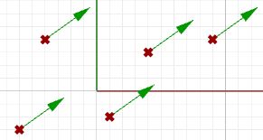
To represent that vector, we need an anchor point in the coordinate system. For example, all of the arrows in the following figure are equal representations of the same vector despite the fact that they are anchored at different locations.

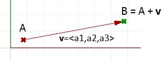
Figure 1: Vector representation in the 3-D coordinate system.

Given a 3D vector v = < a1, a2, a3 >, all vector components a1, a2, a3 are real numbers. Also all line segments from a point A(x,y,z) to point B(x+a1, y+a2, z+a3) are equivalent representations of vector v.

So, how do we define the end points of a line segment that represents a given vector?

Let us define an anchor point (A) so that:

A = (1, 2, 3)

And a vector:

v = <5, 6, 7>

The tip point (B) of the vector is calculated by adding the corresponding components from anchor point and vector v:

B = A + v

B = (1+5, 2+6, 3+7)

B = (6, 8, 10)

Figure 2: The relationship between a vector, the vector anchor point, and the point coinciding with the vector tip location.

Position vector

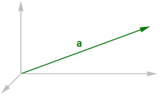
One special vector representation uses the origin point (0,0,0) as the vector anchor point. The position vector v = <a1,a2,a3> is represented with a line segment between two points, the origin and B, so that:

Origin point = (0,0,0)

B = (a1,a2,a3)

Figure 3: Position vector. The tip point coordinates equal the corresponding vector components.

A position vector for a given vector v= < a1,a2,a3 > is a special line segment representation from the origin point (0,0,0) to point (a1,a2,a3).

Vectors vs. points

Do not confuse vectors and points. They are very different concepts. Vectors, as we mentioned, represent a quantity that has direction and length, while points indicate a location. For example, the North direction is a vector, while the North Pole is a location (point).

If we have a vector and a point that have the same components, such as:

v = <3,1,0>

P = (3,1,0)

We can draw the vector and the point as follows:

Figure 4: A vector defines a direction and length. A point defines a location.

Vector length

As mentioned before, vectors have length. We will use |a| to notate the length of a given vector a. For example:

a = <4, 3, 0>

|a| = √(4² + 3² + 0²)

|a| = 5

In general, the length of a vector a<a1,a2,a3> is calculated as follows:

|a| = √(a1² + a2² + a3²)

Figure 5: Vector length.

Unit vector

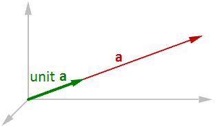
A unit vector is a vector with a length equal to one unit. Unit vectors are commonly used to compare the directions of vectors.

A unit vector is a vector whose length is equal to one unit.

To calculate a unit vector, we need to find the length of the given vector, and then divide the vector components by the length. For example:

|a = <4, 3, 0>

|a| = √(4² + 3² + 0²)

|a| = 5 unit length

If b = unit vector of a, then:

b = <4/5, 3/5, 0/5>

b = <0.8, 0.6, 0>

|b| = √(0.8² + 0.6² + 0²)

|b| = √(0.64 + 0.36 + 0)

|b| = √(1) = 1 unit length

In general:

a = <a1, a2, a3>

The unit vector of a = <a1/|a|, a2/|a|, a3/|a|>

Figure 6: Unit vector equals one-unit length of the vector.

Vector operations

Vector scalar operation

Vector scalar operation involves multiplying a vector by a number. For example:

a = <4, 3, 0>

2*a = <2*4, 2*3, 2*0>

2*a = <8, 6, 0>

Figure 7: Vector scalar operation.

In general, given vector a = <a1, a2, a3>, and a real number t

t*a = < t*a1, t*a2, t*a3 >

Vector addition

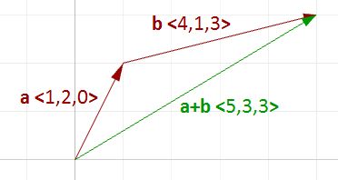
Vector addition takes two vectors and produces a third vector. We add vectors by adding their components.

Vectors are added by adding their components.

For example, if we have two vectors:

a<1, 2, 0>

b<4, 1, 3>

a+b = <1+4, 2+1, 0+3>

a+b = <5, 3, 3>

Figure 8: Vector addition.

In general, vector addition of the two vectors a and b is calculated as follows:

a = <a1, a2, a3>

b = <b1, b2, b3>

a+b = <a1+b1, a2+b2, a3+b3>

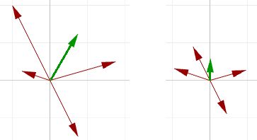
Vector addition is useful for finding the average direction of two or more vectors. In this case, we usually use same-length vectors. Here is an example that shows the difference between using same-length vectors and different-length vectors on the resulting vector addition:

Figure 9: Adding various length vectors (left). Adding same length vectors (right) to get the average direction.

Input vectors are not likely to be same length. In order to find the average direction, you need to use the unit vector of input vectors. As mentioned before, the unit vector is a vector of that has a length equal to 1.

Vector subtraction

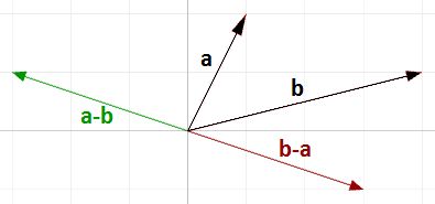
Vector subtraction takes two vectors and produces a third vector. We subtract two vectors by subtracting corresponding components. For example, if we have two vectors a and b and we subtract b from a, then:

a<1, 2, 0>

b<4, 1, 4>

a-b = <1-4, 2-1, 0-4>

a-b = <-3, 1, -4>

If we subtract b from a, we get a different result:

b - a = <4-1, 1-2, 4-0>

b - a = <3, -1, 4>

Note that the vector b - a has the same length as the vector a - b, but goes in the opposite direction.

Figure 10: Vector subtraction.

In general, if we have two vectors, a and b, then a - b is a vector that is calculated as follows:

a = <a1, a2, a3>

b = <b1, b2, b3>

a - b = <a1 - b1, a2 - b2, a3 - b3>

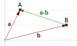
Vector subtraction is commonly used to find vectors between points. So if we need to find a vector that goes from the tip point of the position vector b to the tip point of the position vector a, then we use vector subtraction (a-b) as shown in Figure 11.

Figure 11: Use vector subtraction to find a vector between two points.

Vector properties

There are eight properties of vectors. If a, b, and c are vectors, and s and t are numbers, then:

a + b = b + a

a + 0 = a

s * (a + b) = s * a + s * b

s * t * (a) = s * (t * a)

a + (b + c) = (a + b) + c

a + (-a) = 0

(s + t) * a = s * a + t * a

1 * a = a

Vector dot product

The dot product takes two vectors and produces a number.

For example, if we have the two vectors a and b so that:

a = <1, 2, 3>

b = <5, 6, 7>

Then the dot product is the sum of multiplying the components as follows:

a · b = 1 * 5 + 2 * 6 + 3 * 7

a · b = 38

In general, given the two vectors a and b:

a = <a1, a2, a3>

b = <b1, b2, b3>

a · b = a1 * b1 + a2 * b2 + a3 * b3

We always get a positive number for the dot product between two vectors when they go in the same general direction. A negative dot product between two vectors means that the two vectors go in the opposite general direction.

Figure 12: When the two vectors go in the same direction (left), the result is a positive dot product. When the two vectors go in the opposite direction (right), the result is a negative dot product.

When calculating the dot product of two unit vectors, the result is always between 1 and +1. For example:

a = <1, 0, 0>

b = <0.6, 0.8, 0>

a · b = (1 * 0.6, 0 * 0.8, 0 * 0) = 0.6

In addition, the dot product of a vector with itself is equal to that vector’s length to the power of two. For example:

a = <0, 3, 4>

a · a = 0 * 0 + 3 * 3 + 4 * 4

a · a = 25

Calculating the square length of vector a:

| a | = √(4² + 3² + 0²)

| a | = 5

| a |² = 25

Vector dot product, lengths, and angles

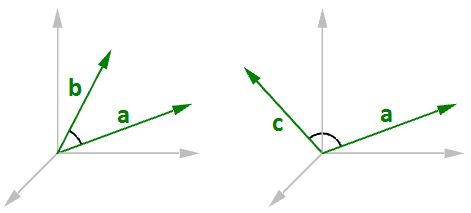
There is a relationship between the dot product of two vectors and the angle between them.

The dot product of two non-zero unit vectors equals the cosine of the angle between them.

In general:

a · b = | a | * | a | * cos(ө), or

a · b / (| a | * | a |) = cos(ө)

Where:

ө is the angle included between the vectors.

If vectors a and b are unit vectors, we can simply say:

a · b = cos(ө)

And since the cosine of a 90-degree angle is equal to 0, we can say:

Vectors a and b are orthogonal if, and only if, a · b = 0.

For example, if we calculate the dot product of the two orthogonal vectors, World xaxis and yaxis, the result will equal zero.

x = <1, 0, 0>

y = <0, 1, 0>

x · y = (1 * 0) + (0 * 1) + (0 * 0)

x · y = 0

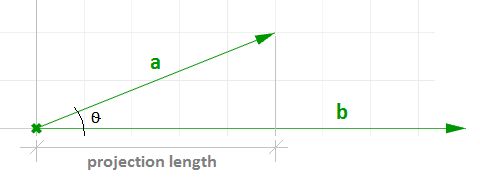
There is also a relationship between the dot product and the projection length of one vector onto another. For example:

a = <5, 2, 0>

b = <9, 0, 0>

unit(b) = <1, 0, 0>

a · unit(b) = (5 * 1) + (2 * 0) + (0 * 0)

a · unit(b) = 2 (which is equal to the projection length of a onto b)

Figure 13: The dot product equals the projection length of one vector onto a non-zero unit vector.

In general, given a vector a and a non-zero vector b, we can calculate the projection length pL of vector a onto vector b using the dot product.

pL = |a| * cos(ө)

pL = a · unit(b)

Dot product properties

If a, b, and c are vectors and s is a number, then:

a · a = | a |²

a · (b + c) = a · b + a · c

0 · a = 0

a · b = b · a

(s * a) · b = s * (a · a) = a · (s * b)

Vector cross product

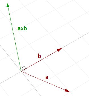
The cross product takes two vectors and produces a third vector that is orthogonal to both.

Figure 14: Calculating the cross product of two vectors.

For example, if you have two vectors lying on the World xy-plane, then their cross product is a vector perpendicular to the xy-plane going either in the positive or negative World z-axis direction. For example:

a = <3, 1, 0>

b = <1, 2, 0>

a × b = < (1 * 0 – 0 * 2), (0 * 1 - 3 * 0), (3 * 2 - 1 * 1) >

a × b = <0, 0, 5>

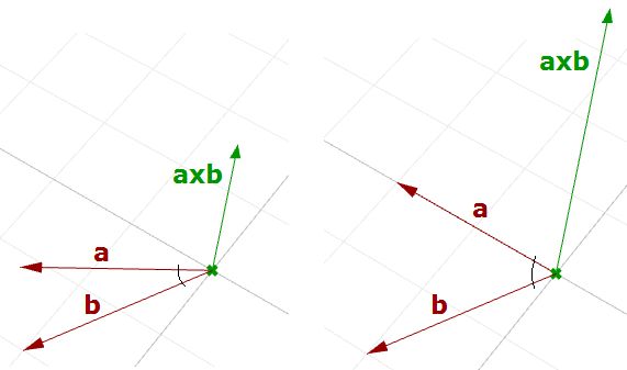
The vector a x b is orthogonal to both a and b.

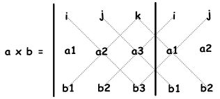
You will probably never need to calculate a cross product of two vectors by hand, but if you are curious about how it is done, continue reading; otherwise you can safely skip this section. The cross product a × b is defined using determinants. Here is a simple illustration of how to calculate a determinant using the standard basis vectors:

i = <1, 0, 0>

j = <0,1, 0>

k = <0, 0, 1>

The cross product of the two vectors a<a1, a2, a3> and b<b1, b2, b3> is calculated as follows using the above diagram:

a × b = i (a2 * b3) + j (a3 * b1) + k (a1 * b2) - k (a2 * b1) - i (a3 * b2) - j (a1 * b3)

a × b = i (a2 * b3 - a3 * b2) + j (a3 * b1 - a1 * b3) + k (a1 * b2 - a2 * b1)

a × b = <a2 * b3 – a3 * b2, a3 * b1 - a1 * b3, a1 * b2 - a2 * b1 >

Cross product and angle between vectors

There is a relationship between the angle between two vectors and the length of their cross product vector. The smaller the angle (smaller sine); the shorter the cross product vector will be. The order of operands is important in vectors cross product. For example:

a = <1, 0, 0>

b = <0, 1, 0>

a × b = <0, 0, 1>

b × a = <0, 0, -1>

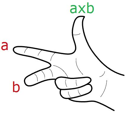
Figure 15: The relationship between the sine of the angle between two vectors and the length of their cross product vector.

In Rhino's right-handed system, the direction of a × b is given by the right-hand rule (where a = index finger, b = middle finger, and a × b = thumb).

In general, for any pair of 3-D vectors a and b:

| a × b | = | a | | b | sin(ө)

Where:

ө is the angle included between the position vectors of a and b

If a and b are unit vectors, then we can simply say that the length of their cross product equals the sine of the angle between them. In other words:

| a × b | = sin(ө)

The cross product between two vectors helps us determine if two vectors are parallel. This is because the result is always a zero vector.

Vectors a and b are parallel if, and only if, a x b = 0.

Cross product properties

If a, b, and c are vectors, and s is a number, then:

a × b = -b × a

(s * a) × b = s * (a × b) = a × (s * b)

a × (b + c) = a × b + a × c

(a + b) × c = a × c + b × c

a · (b × c) = (a × b) · c

a × (b × c) = (a · c) * b – (a · b) * c

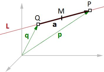
Vector equation of line

The vector line equation is used in 3D modeling applications and computer graphics.

Figure 16: Vector equation of a line.

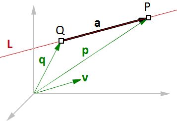
For example, if we know the direction of a line and a point on that line, then we can find any other point on the line using vectors, as in the following:

L = line

v = <a, b, c> line direction unit vector

Q = (x0, y0, z0) line position point

P = (x, y, z) any point on the line

We know that:

a = t * v --- (2)

p = q + a --- (1)

From 1 and 2:

p = q + t * v --- (3)

However, we can write (3) as follows:

<x, y, z> = <x0, y0, z0> + <t * a, t * b, t * c>

<x, y, z> = <x0 + t * a, y0 + t * b, z0 + t * c>

Therefore:

x = x0 + t * a

y = y0 + t * b

z = z0 + t * c

Which is the same as:

P = Q + t * v

Given a point Q and a direction v on a line, any point P on that line can be calculated using the vector equation of a line P = Q + t * v where t is a number.

Another common example is to find the midpoint between two points. The following shows how to find the midpoint using the vector equation of a line:

q is the position vector for point Q

p is the position vector for point P

a is the vector going from Q to P

From vector subtraction, we know that:

a = p - q

From the line equation, we know that:

M = Q + t * a

And since we need to find midpoint, then:

t = 0.5

Hence we can say:

M = Q + 0.5 * a

Figure 17: Find the midpoint between two input points.

In general, you can find any point between Q and P by changing the t value between 0 and 1 using the general equation:

M = Q + t * (P - Q)

Given two points Q and P, any point M between the two points is calculated using the equation M = Q + t * (P - Q) where t is a number between 0 and 1.

Vector equation of a plane

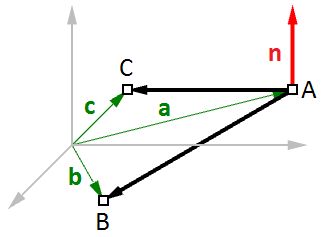
One way to define a plane is when you have a point and a vector that is perpendicular to the plane. That vector is usually referred to as normal to the plane. The normal points in the direction above the plane.

One example of how to calculate a plane normal is when we know three non-linear points on the plane.

In Figure 18, given:

A = the first point on the plane

B = the second point on the plane

C = the third point on the plane

And:

a = a position vector of point A

b = a position vector of point B

c = a position vector of point C

We can find the normal vector n as follows:

n = (b - a) × (c - a)

Figure 18: Vectors and planes.

We can also derive the scalar equation of the plane using the vector dot product:

n · (b - a) = 0

If:

n = <a, b, c>

b = <x, y, z>

a = <x0, y0, z0>

Then we can expand the above:

<a, b, c> · <x-x0, y-y0, z-z0 > = 0

Solving the dot product gives the general scalar equation of a plane:

a * (x - x0) + b * (y - y0) + c * (z - z0) = 0

Tutorials

All the concepts we reviewed in this chapter have a direct application to solving common geometry problems encountered when modeling. The following are step by step tutorials that use the concepts learned in this chapter using Rhinoceros and Grasshopper (GH).

Face direction

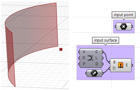
Given a point and a surface, how can we determine whether the point is facing the front or back side of that surface?

Input
1: A surface 2: A point
Parameters
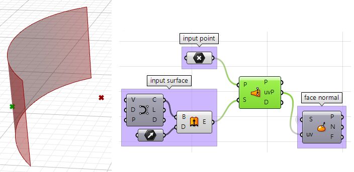
The face direction is defined by the surface normal direction. We will need the following information: ● The surface normal direction at a surface location closest to the input point. ● A vector direction from the closest point to the input point. Compare the above two directions, if going the same direction, the point is facing the front side, otherwise it is facing the back.
Solution
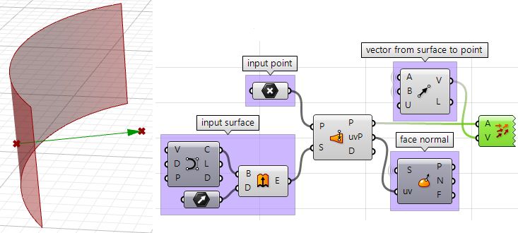
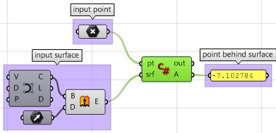
1: Find the closest point location on the surface relative to the input point using the Pull component. This will give us the uv location of the closest point, which we can then use to evaluate the surface and find its normal direction.
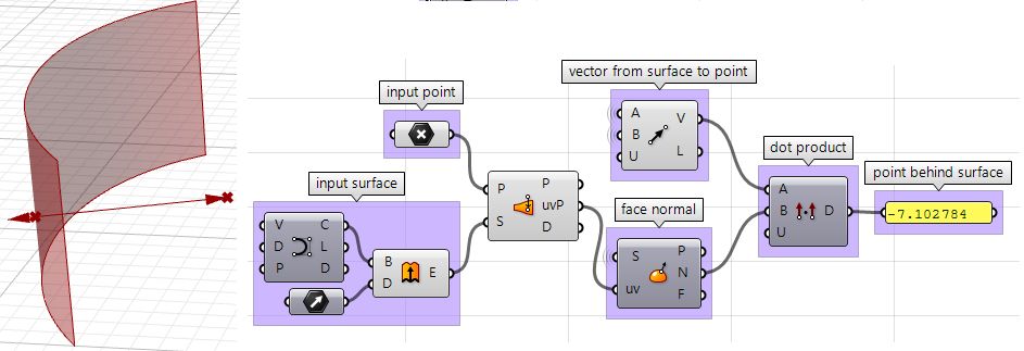
2: We can now use the closest point to draw a vector going towards the input point. We can also draw:
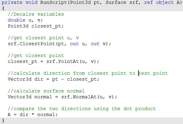
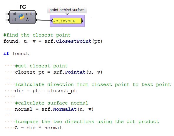
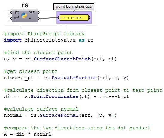
3: We can compare the two vectors using the dot product. If the result is positive, the point is in front of the surface. If the result is negative, the point is behind the surface.

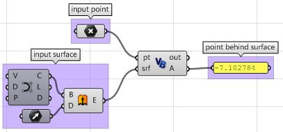
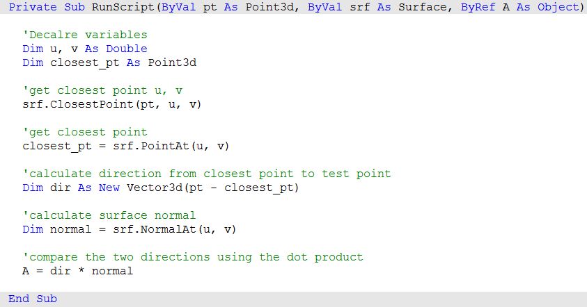
The above steps can also be solved using other scripting languages.

Using the Grasshopper VB component

Using the Grasshopper C# component

Using the Grasshopper Python component and the RhinoCommon SDK

Using the Grasshopper Python component and the RhinoScriptSyntax Library

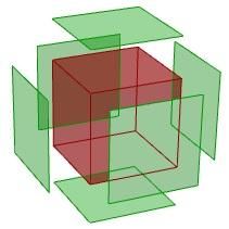
Exploded box

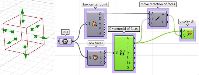
The following tutorial shows how to explode a polysurface. This is what the final exploded box looks like:

Input
Identify the input, which is a box. We will use the Box parameter in GH.
Parameters
Think of all the parameters we need to know in order to solve this tutorial. ● The center of explosion. ● The box faces we are exploding. ● The direction in which each face is moving. Once we have identified the parameters, it is a matter of putting it together in a solution by piecing together the logical steps to reach an answer.
Solution
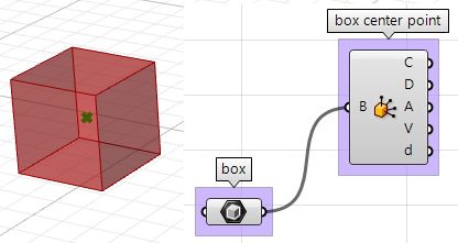
1: Find the center of the box using the Box Properties component in GH:
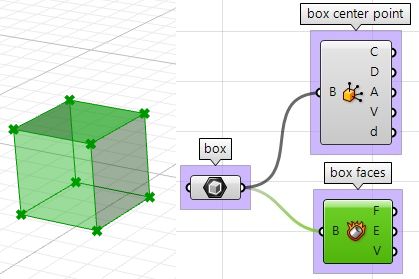
2: Extract the box faces with the Deconstruct Brep component:
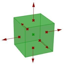
3: The direction we move the faces is the tricky part. We need to first find the center of each face, and then define the direction from the center of the box towards the center of each face as follows:
4: Once we have all the parameters scripted, we can use the Move component to move the faces in the appropriate direction. Just make sure to set the vectors to the desired amplitude, and you will be good to go.

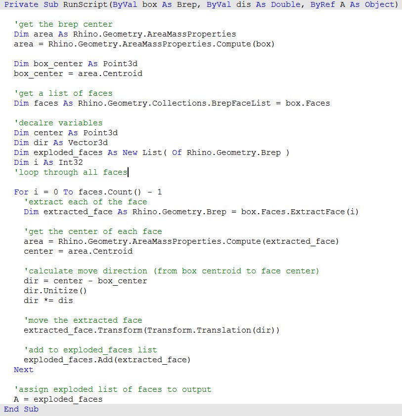
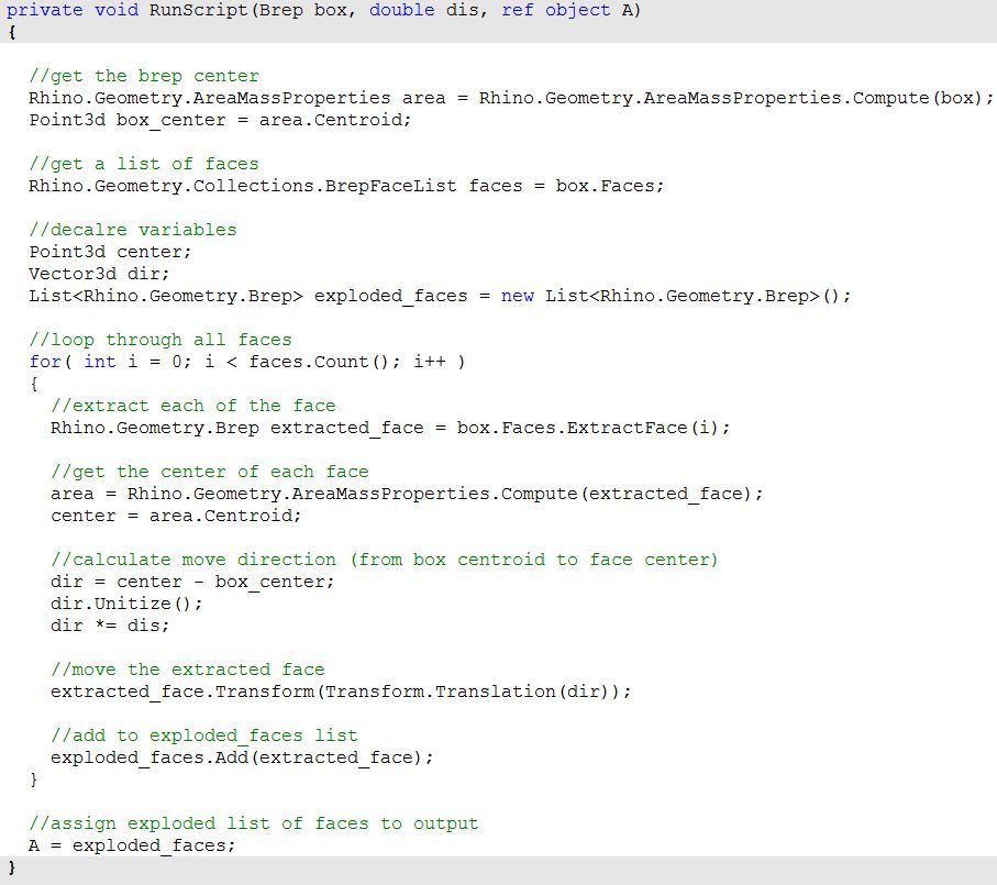
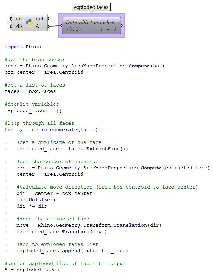
The above steps can also be solved using VB script, C# or Python. Following is the solution using these scripting languages.

Using the Grasshopper VB component

Using the Grasshopper C# component

Using the Grasshopper Python component

Tangent spheres

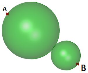
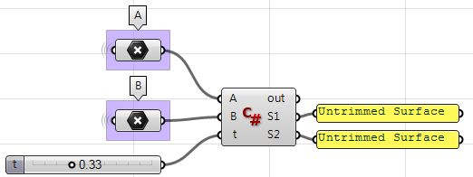
This tutorial will show how to create two tangent spheres between two input points. This is what the result looks like:

Input
Two points (A and B) in the 3-D coordinate system.
Parameters
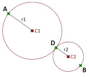
The following is a diagram of the parameters that we will need in order to solve the problem: ● A tangent point D between the two spheres, at some t parameter (0-1) between points A and B. ● The center of the first sphere or the midpoint C1 between A and D. ● The center of the second sphere or the midpoint C2 between D and B. ● The radius of the first sphere (r1) or the distance between A and C1. ● The radius of the second sphere (r2) or the distance between D and C2.
Solution
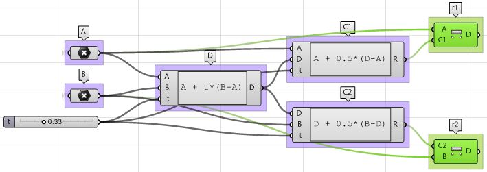
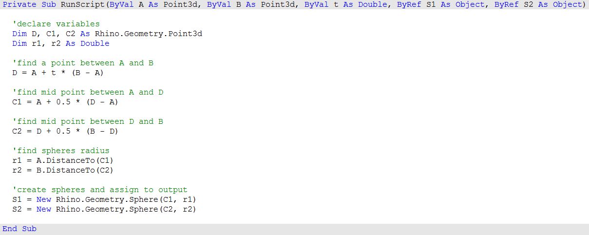
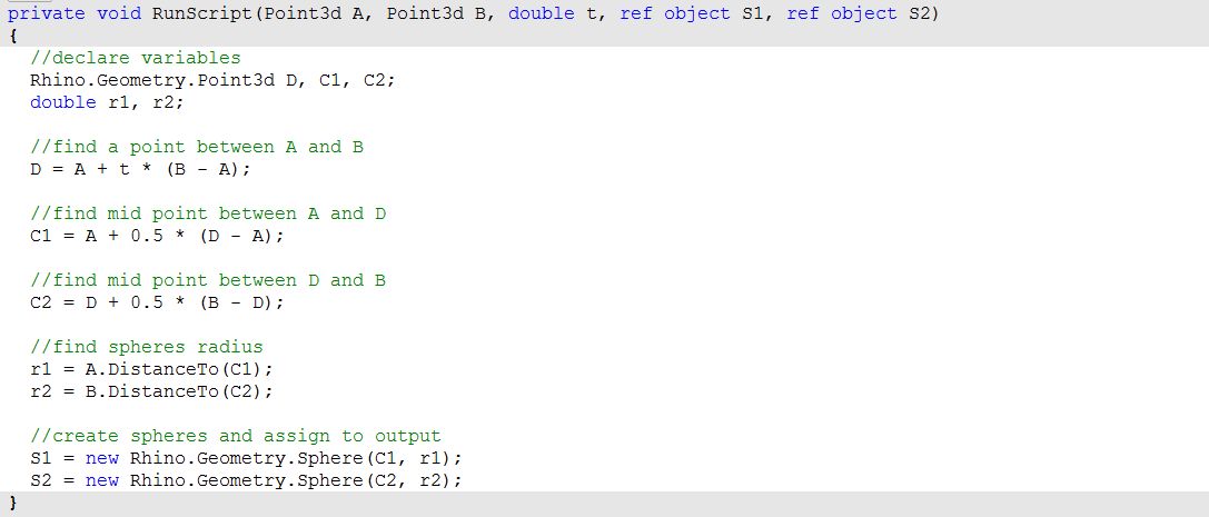
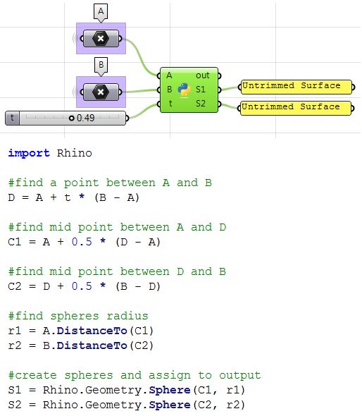
1: Use the Expression component to define point D between A and B at some parameter t. The expression we will use is based on the vector equation of a line: D = A + t(B-A). ● B-A: is the vector that goes from B to A using the vector subtraction operation. ● t(B-A): where t is between 0 and 1 to get us a location on the vector. ● A+t*(B-A): gets a point on the vector between A and B.
2: Use the Expression component to also define the mid points C1 and C2.
3: The first sphere radius (r1) and the second sphere radius (r2) can be calculated using the Distance component.
4: The final step involves creating the sphere from a base plane and radius. We need to make sure the origins are hooked to C1 and C2 and the radius from r1 and r2.

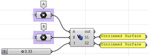
The above steps can also be solved as follows.

Using the Grasshopper VB component

Using the Grasshopper C# component

Using the Grasshopper Python component

Matrices and Transformations

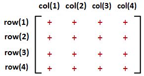
Transformations refer to operations such as moving (also called translating), rotating, and scaling objects. They are stored in 3D programming using matrices, which are nothing but rectangular arrays of numbers. Multiple transformations can be performed very quickly using matrices. It turns out that a [4x4] matrix can represent all transformations. Having a unified matrix dimension for all transformations saves calculation time.

Matrix operations

The one operation that is most relevant in computer graphics is matrix multiplication. We will explain it with some detail.

Matrix multiplication

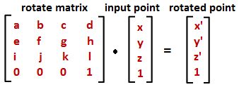
Matrix multiplication is used to apply transformations to geometry. For example if we have a point and would like to rotate it around some axis, we use a rotation matrix and multiply it by the point to get the new rotated location.

Most of the time, we need to perform multiple transformations on the same geometry. For example, if we need to move and rotate a thousand points, we can use either of the following methods.

Method 1
1. Multiply the move matrix by 1000 points to move the points. 2. Multiply the rotate matrix by the resulting 1000 points to rotate the moved points. Number of operations = 2000.
Method 2
1. Multiply the rotate and move matrices to create a combined transformation matrix. 2. Multiply the combined matrix by 1000 points to move and rotate in one step. Number of operations = 1001.

Notice that method 1 takes almost twice the number of operations to achieve the same result. While method 2 is very efficient, it is only possible if both the move and rotate matrices are [4x4]. This is why in computer graphics a [4x4] matrix is used to represent all transformations, and a [4x1] matrix is used to represent points.

Three-dimensional modeling applications provide tools to apply transformations and multiply matrices, but if you are curious about how to mathematically multiply matrices, we will explain a simple example. In order to multiply two matrices, they have to have matching dimensions. That means the number of columns in the first matrix must equal the number of rows of the second matrix. The resulting matrix has a size equal to the number of rows from the first matrix and the number of columns from the second matrix. For example, if we have two matrices, M and P, with dimensions equal to [4x4] and [4x1] respectively, then there resulting multiplication matrix M · P has a dimension equal to [4x1] as shown in the following illustration:

Identity matrix

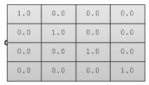
The identity matrix is a special matrix where all diagonal components equal 1 and the rest equal 0.

The main property of the identity matrix is that if it is multiplied by any other matrix, the values multiplied by zero do not change.

Transformation operations

Most transformations preserve the parallel relationship among the parts of the geometry. For example collinear points remain collinear after the transformation. Also points on one plane stay coplanar after transformation. This type of transformation is called an affine transformation.

Translation (move) transformation

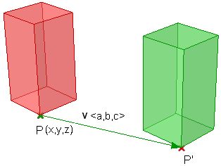
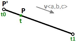
Moving a point from a starting position by certain a vector can be calculated as follows:

P' = P + V

Suppose:

P(x,y,z) is a given point

v<a,b,c> is a translation vector

Then:

P'(x) = x + a

P'(y) = y + b

P'(z) = z + c

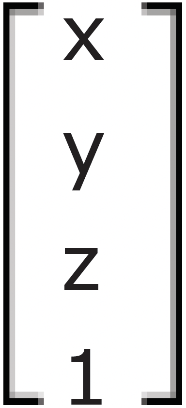
Points are represented in a matrix format using a [4x1] matrix with a 1 inserted in the last row. For example the point P(x,y,z) is represented as follows:

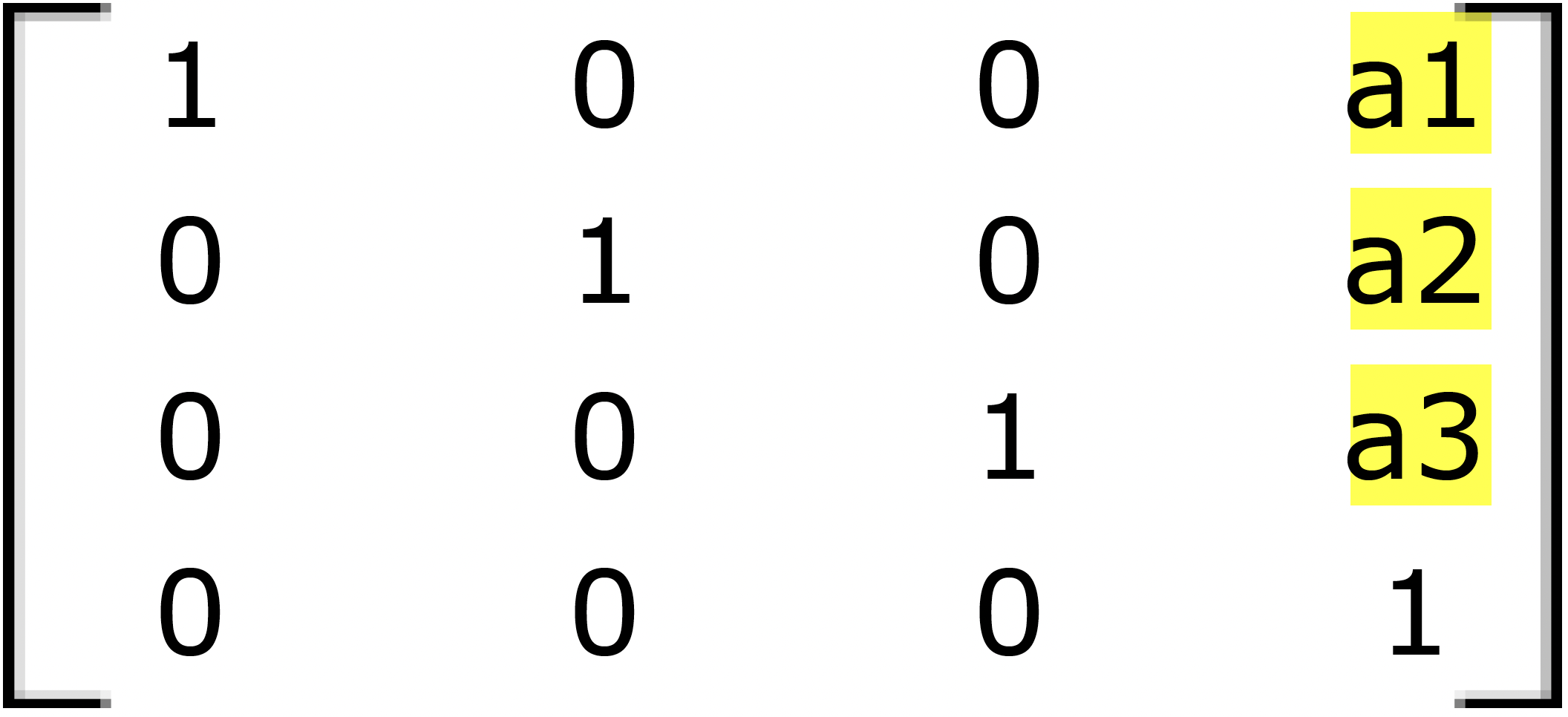
Using a [4x4] matrix for transformations (what is called a homogenous coordinate system), instead of a [3x3] matrices, allows representing all transformations including translation. The general format for a translation matrix is:

For example, to move point P(2,3,1) by vector v<2,2,2>, the new point location is:

P’ = P + v = (2+2, 3+2, 1+2) = (4, 5, 3)

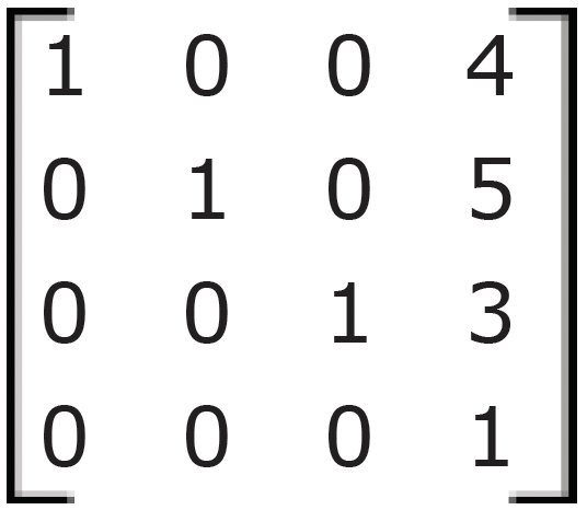
If we use the matrix form and multiply the translation matrix by the input point, we get the new point location as in the following:

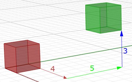
Similarly, any geometry is translated by multiplying its construction points by the translation matrix. For example, if we have a box that is defined by eight corner points, and we want to move it 4 units in the x-direction, 5 units in the y-direction and 3 units in the z- direction, we must multiply each of the eight box corner points by the following translation matrix to get the new box.

Figure 19: Translate all box corner points.

Rotation transformation

This section shows how to calculate rotation around the z-axis and the origin point using trigonometry, and then to deduce the general matrix format for the rotation.

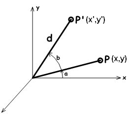
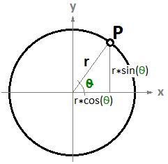
Take a point on x,y plane P(x,y) and rotate it by angle(b).

From the figure, we can say the following:

x = d cos(a) ---(1)

y = d sin(a) ---(2)

x' = d cos(b+a) ---(3)

y' = d sin(b+a) --- (4)

Expanding x' and y' using trigonometric identities for the sine and cosine of the sum of angles:

x' = d cos(a)cos(b) - d sin(a)sin(b) ---(5)

y' = d cos(a)sin(b) + d sin(a)cos(b) ---(6)

Using Eq 1 and 2:

x' = x cos(b) - y sin(b)

y' = x sin(b) + y cos(b)

The rotation matrix around the z-axis looks like:

The rotation matrix around the x-axis by angle b looks like:

The rotation matrix around the y-axis by angle b looks like:

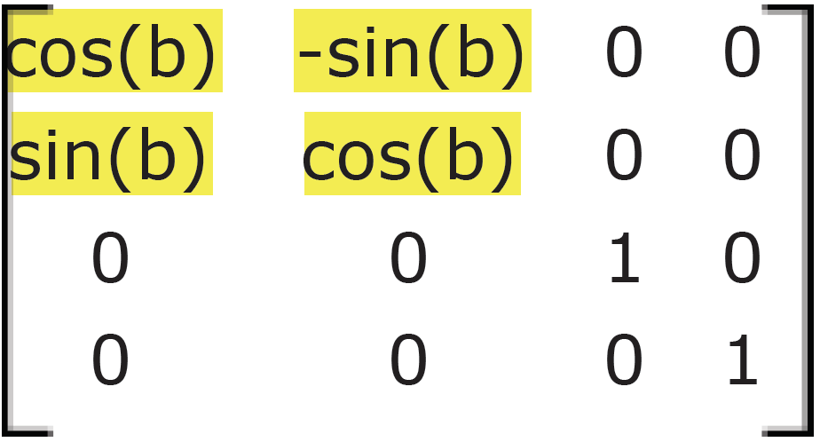
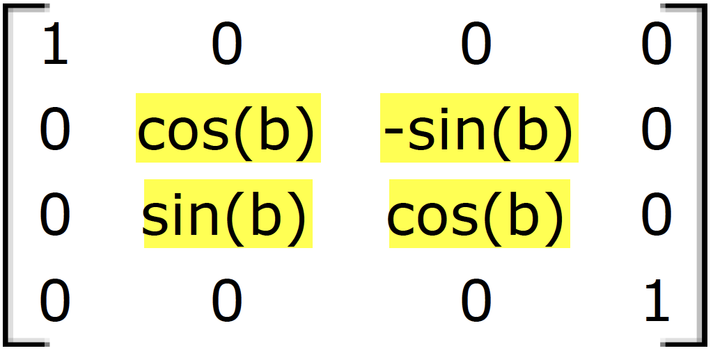
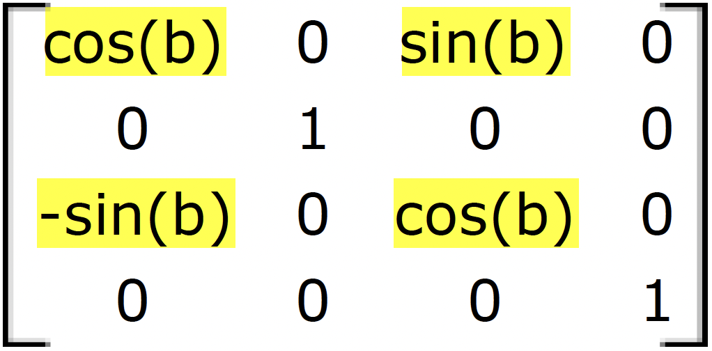
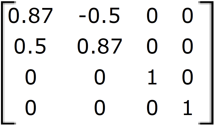
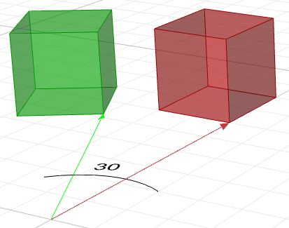
For example, if we have a box and would like to rotate it 30 degrees, we need the following:

1. Construct the 30-degree rotation matrix. Using the generic form and the cos and sin values of 30-degree angle, the rotation matrix will look like the following:
2. Multiply the rotation matrix by the input geometry, or in the case of a box, multiply by each of the corner points to find the box's new location.

Figure 20: Rotate geometry.

Scale transformation

In order to scale geometry, we need a scale factor and a center of scale. The scale factor can be uniform scaling equally in x-, y-, and z-directions, or can be unique for each dimension.

Scaling a point can use the following equation:

P' = ScaleFactor(S) * P

Or:

P'.x = S_x * P.x

P'.y = S_y * P.y

P'.z = S_z * P.z

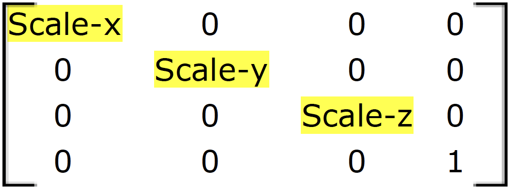
This is the matrix format for scale transformation, assuming that the center of scale is the World origin point (0,0,0):

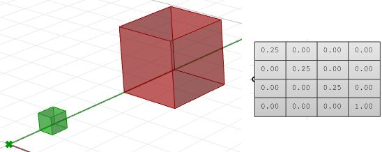
For example, if we would like to scale a box by 0.25 relative to the World origin, the scale matrix will look like the following:

Figure 21: Scale geometry.

Shear transformation

Shear in 3D is measured along a pair of axes relative to a third axis. For example, a shear along a zaxis will not change geometry along that axis, but will alter it along x and y. Here are few examples of shear matrices:

1. Shear in x and z, keeping the y-coordinate fixed:

2. Shear in y and z, keeping the x-coordinate fixed:

3. Shear in x and y, keeping the z-coordinate fixed:

Figure 22: Shear Matrices.

Mirror or reflection transformation

The mirror transformation creates a reflection of an object across a line or a plane. 2-D objects are mirrored across a line, while 3-D objects are mirrored across a plane. Keep in mind that the mirror transformation flips the normal direction of the geometry faces.

Planar Projection transformation

Intuitively, the projection point of a given 3-D point P(x,y,z) on the world xy-plane equals P_xy(x,y,0) setting the z value to zero. Similarly, a projection to xz-plane of point P is P_xz(x,0,z). When projecting to yz-plane, P_xz = (0,y,z). Those are called [[Bézier curve|orthogonal projections]].

If we have a curve as an input, and we apply the planar projection transformation, we get a curve projected to that plane. The following shows an example of a curve projected to xyplane with the matrix format.

Note: NURBS curves (explained in the next chapter) use control points to define curves. Projecting a curve amounts to projecting its control points.

Figure 24: Projection matrices.

Tutorial

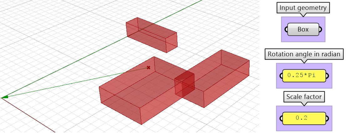
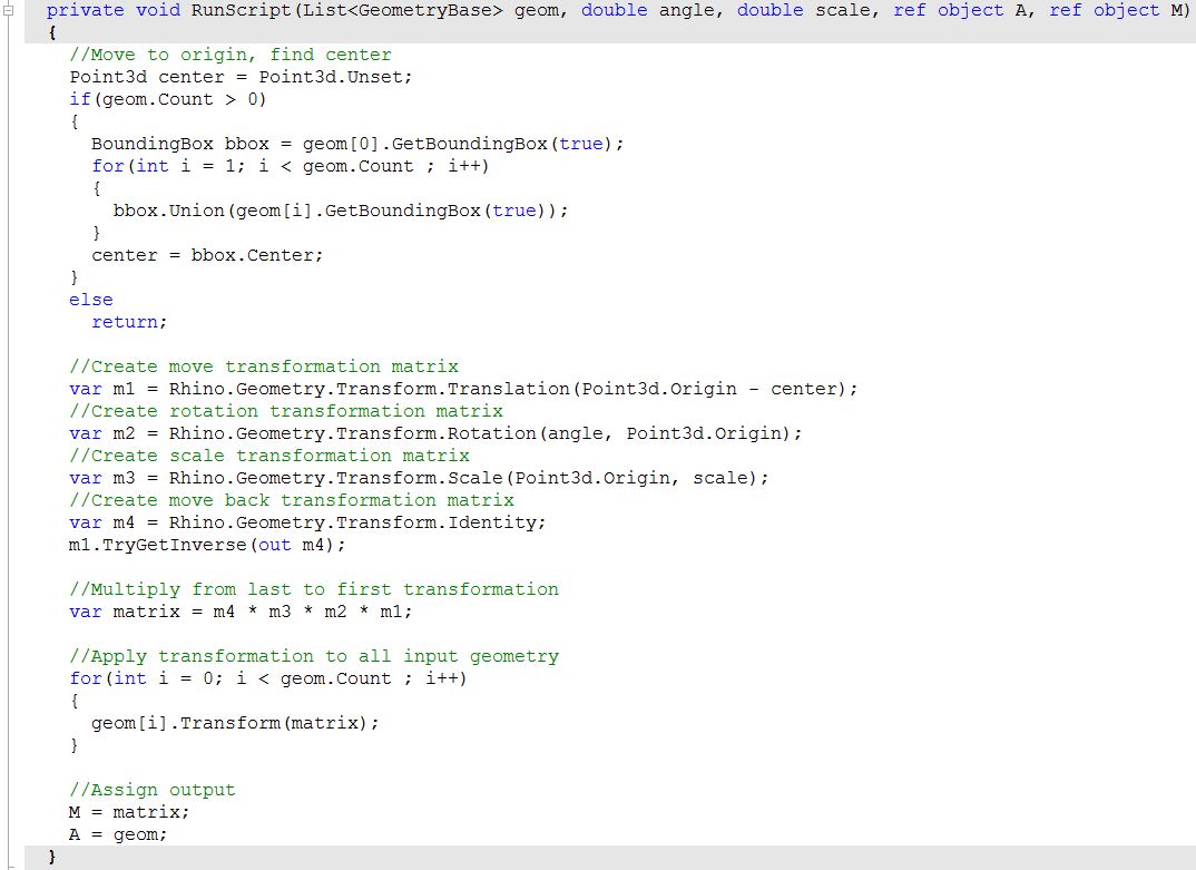
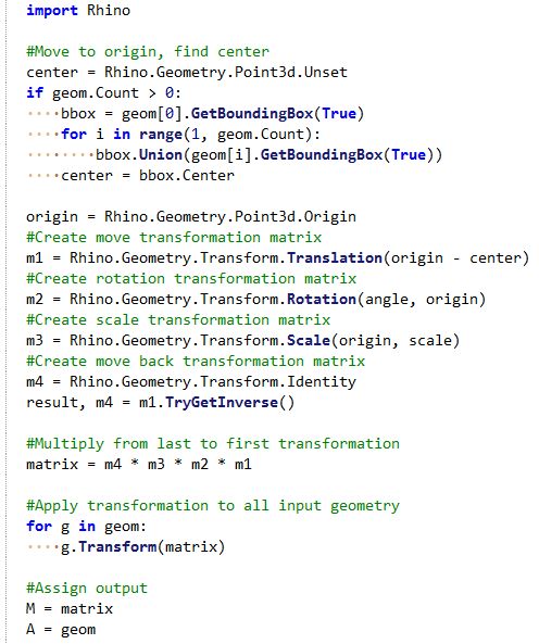
Multiple transformations

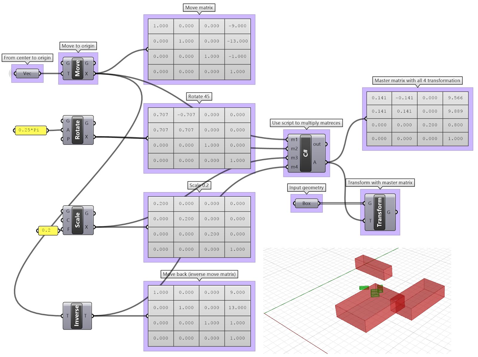
Use one matrix to transform geometry as follows:

First, move input geometry so that it's center is at the origin, then rotate 45 degrees around the z axis, then scale uniformly by 0.2, then move back to original location.

Performance note: With big number of points or objects to transform, it is much more efficient to create one master transformation matrix (multiply all matrices first), then use resulting master matrix once to transform all input, as opposed to transforming multiple times with one matrix at a time.

Input
1: Objects to transform 2: Rotation angle (45 degrees) and scale factor (0.2).
Additional Input
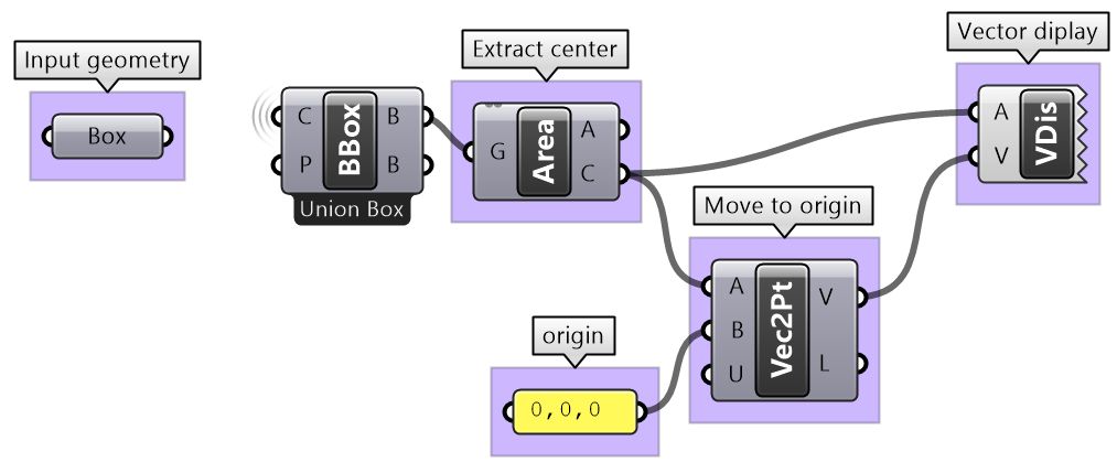
Initial move needs the following: ● Vector from the bounding box center of input to origin.
Solution
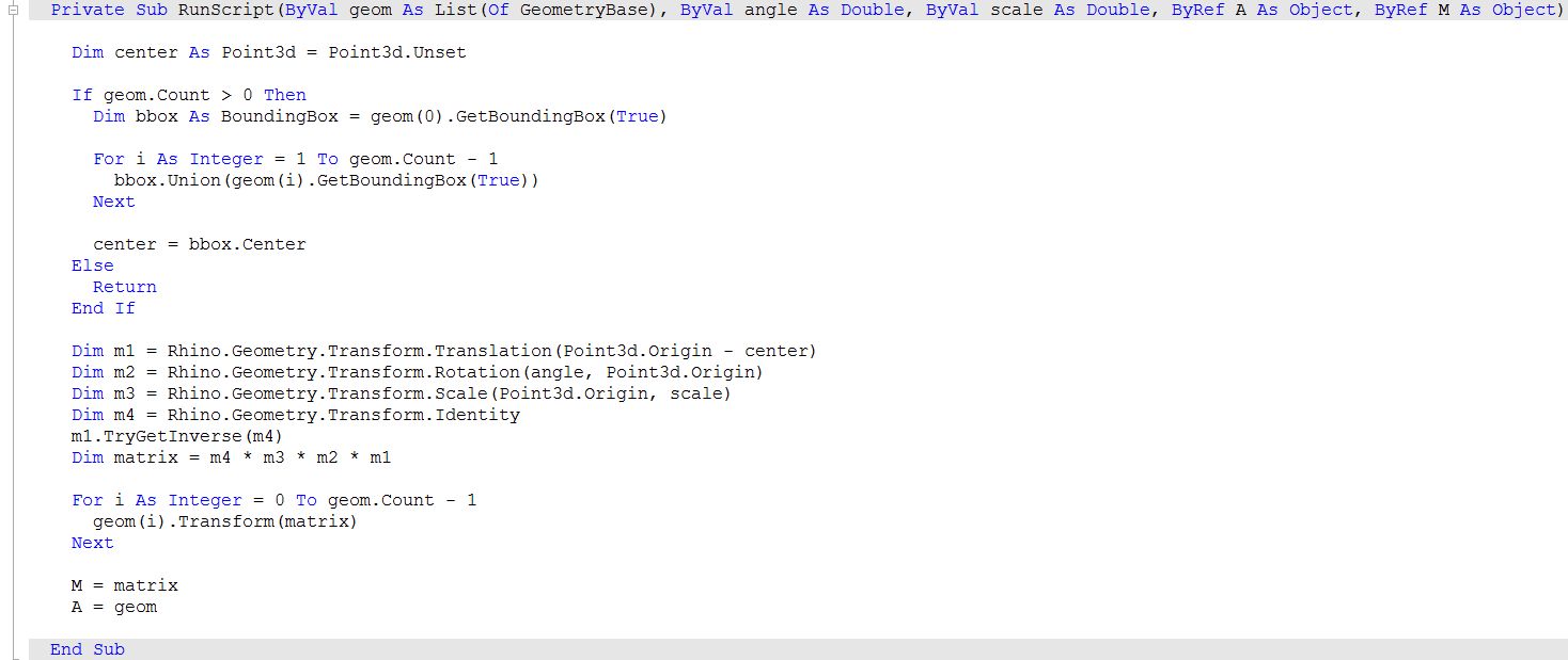
1. Generate all transform matrices: move, rotate, scale and Inverse of initial move. 2. Multiply the matrices from last to first to generate master transformation matrix 3. Transform input using the master transformation matrix.

The above steps can also be solved using scripting.

Using the Grasshopper VB component

Using the Grasshopper C# component

Using the Grasshopper Python component and the RhinoCommon SDK

Parametric Curves and Surfaces

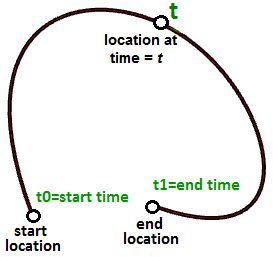
Suppose you travel every weekday from your house to your work. You leave at 8:00 in the morning and arrive at 9:00. At each point in time between 8:00 and 9:00, you would be at some location along the way. If you plot your location every minute during your trip, you can define the path between home and work by connecting the 60 points you plotted. Assuming you travel the exact same speed every day, at 8:00 you would be at home (start location), at 9:00 you would be at work (end location) and at 8:40 you would at the exact same location on the path as the 40th plot point.

Congratulations, you have just defined your first parametric curve! You have used time as a parameter to define your path, and hence you can call your path curve a parametric curve. The time interval you spend from start to end (8 to 9) is called the curve domain or interval.

In general, we can describe the x, y, and z location of a parametric curve in terms of some parameter t as follows:

x = x(t)

y = y(t)

z = z(t)

Where:

t is a range of real numbers.

We saw earlier that the parametric equation of a line in terms of parameter t is defined as:

x = x’ + t * a

y = y’ + t * b

z = z’ + t * c

Where:

x, y, and z are functions of t where t represents a range of real numbers.

X’, y’, and z’ are the coordinates of a point on the line segment.

a, b, and c define the slope of the line, such that the vector v<a, b, c> is parallel to the line.

We can therefore write the parametric equation of a line segment using a t parameter that ranges between two real number values t0, t1 and a unit vector v that is in the direction of the line as follows:

P = P’ + t * v

Another example is a circle. The parametric equation of the circle on the xy-plane with a center at the origin (0,0) and an angle parameter t ranging between 0 and 2π radians is:

x = r cos(t)

y = r sin(t)

We can derive the general equation of a circle for the parametric one as follows:

x/r = cos(t)

y/r = sin(t)

And since:

cos(t)² + sin(t)² = 1 (Pythagorean identity)

Then:

(x/r)² + (y/r)² = 1, or

x² + y² = r²

Parametric curves

Curve parameter

A parameter on a curve represents the address of a point on that curve. As mentioned before, you can think of a parametric curve as a path traveled between two points in a certain amount of time, traveling at a fixed or variable speed. If traveling takes T amount of time, then the parameter t represents a time within T that translates to a location (point) on the curve.

If you have a straight path (line segment) between the two points A and B, and v were a vector from A to B (v = B - A), then you can use the parametric line equation to find all points M between A and B as follows:

M = A + t*(B-A)

Where:

t is a value between 0 and 1.

The range of t values, 0 to 1 in this case, is referred to as the curve domain or interval. If t was a value outside the domain (less than 0 or more than 1), then the resulting point M will be outside the linear curve AB.

Figure 25: Parametric line in 3-D space and parameter interval.

The same principle applies for any parametric curve. Any point on the curve can be calculated using the parameter t within the interval or domain of values that define the limits of the curve. The start parameter of the domain is usually referred to as t0 and the end of the domain as t1.

Figure 26: Curve in 3-D space and its domain in parameter space.

Curve domain or interval

A curve domain or interval is defined as the range of parameters that evaluate into a point within that curve. The domain is usually described with two real numbers defining the domain limits expressed in the form (min to max) or (min, max). The domain limits can be any two values that may or may not be related to the actual length of the curve. In an increasing domain, the domain min parameter evaluates to the start point of the curve and the domain max evaluates to the end point of the curve.

Figure 27: Curve domain or interval is a set of two numbers that is usually ascending. When possible, domain length is set to be close to the 3d curve length, but it can be set to any length without changing the 3d curve.

Changing a curve domain is referred to as the process of reparameterizing the curve. For example, it is very common to change the domain to be (0 to 1).

Reparameterizing a curve does not affect the shape of the 3-D curve. It is like changing the travel time on a path by running instead of walking, which does not change the shape of the path.

Figure 28: Curve domain can be normalized (set to 0 to 1). Note that if the 3d curve length is much bigger than the domain length (by a factor of 10 or more), the evaluation of a parameter might not yield very accurate location on the 3d curve.

An increasing domain means that the minimum value of the domain points to the start of the curve. Domains are typically increasing, but not always.

Curve evaluation

We learned that a curve interval is the range of all parameter values that evaluate to points within the 3-D curve. There is, however, no guarantee that evaluating at the middle of the domain, for example, will give a point that is in the middle of the curve.

We can think of uniform parameterization of a curve as traveling a path with constant speed. A degree-1 line between two points is one example where equal intervals or parameters translate into equal intervals of arc length on the line as in figure (29). In parametric curves, it is rare that equal intervals of parameters evaluate to equal intervals on the 3-D curve.

Figure 29: A special case of a degree-1 line where equal parameter intervals, evaluate to equal curve lengths.

It is more likely that the speed decreases or increases along the path. For example, if it takes 30 minutes to travel a road, it is unlikely that you will be exactly half way through at minute 15. Figure (30) shows a typical case where equal parameter intervals evaluate to variable length on the 3-D curve.

Figure 30: Equal parameter intervals do not usually translate into equal distances on a parametric curves such as NURBS curves.

You may need to evaluate points on a 3-D curve that are at a defined percentage of the curve length. For example, you might need to divide the curve into equal lengths. Typically, 3-D modelers provide tools to evaluate curves relative to arc length.

Tangent vector to a curve

A tangent to a curve at any parameter (or point on a curve) is the vector that touches the curve at that point, but does not cross over. The slope of the tangent vector equals the slope of the curve at the same point. The following example evaluates the tangent to a curve at two different parameters.

Figure 31: Tangents to a curve.

Cubic polynomial curves

Hermite and Bézier curves are two examples of cubic polynomial curves that are determined by four parameters. A Hermite curve is determined by two end points and two tangent vectors at these points, while a Bézier curve is defined by four points. While they differ mathematically, they share similar characteristics and limitations.

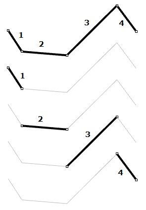
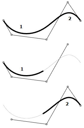
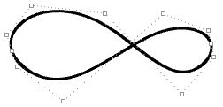
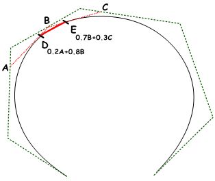
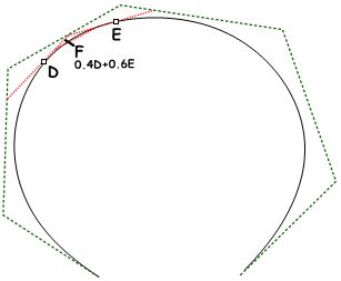
Figure 32: Cubic polynomial curves. The Bézier curve (left) is defined by four points. The Hermite curve (right) is defined by two points and two tangents.

In most cases, curves are made out of multiple segments. This requires making what is called a piecewise cubic curve. Here is an illustration of a piecewise Bézier curve that uses 7 storage points to create a two-segment cubic curve. Note that although the final curve is joined, it does not look smooth or continuous.

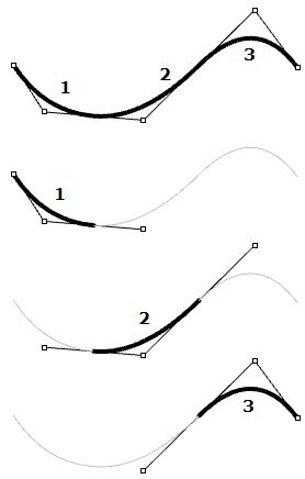
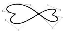
Figure 33: Two Bezier spans share one point.

Although Hermite curves use the same number of parameters as Bézier curves (four parameters to define one curve), they offer the additional information of the tangent curve that can also be shared with the next piece to create a smoother looking curve with less total storage, as shown in the following.

Figure 34: Two Hermite spans share one point and a tangent.

The non-uniform rational B-spline (NURBS) is a powerful curve representation that maintains even smoother and more continuous curves. Segments share more control points to achieve even smoother curves with less storage.

Figure 35: Two degree-3 NURBS spans share three control points.

NURBS curves and surfaces are the main mathematical representation used by Rhino to represent geometry. NURBS curve characteristics and components will be covered with some detail later in this chapter.

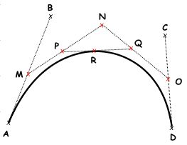
Evaluating cubic Bézier curves

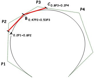
Named after its inventor, Paul de Casteljau, the de Casteljau algorithm evaluates Bézier curves using a recursive method. The algorithm steps can be summarized as follows:

Input
Four points A, B, C, D define a curve t, is any parameter within curve domain.
Output
Point R on curve that is at parameter t.
Solution
1. Find point M at t parameter on line AB. 2. Find point N at t parameter on line BC. 3. Find point O at t parameter on line CD. 4. Find point P at t parameter on line MN. 5. Find point Q at t parameter on line NO. 6. Find point R at t parameter on line PQ.

NURBS curves

NURBS is an accurate mathematical representation of curves that is highly intuitive to edit. It is easy to represent free-form curves using NURBS and the control structure makes it easy and predictable to edit.

Figure 36: Non-uniform rational B-splines and their control structure.

There are many books and references for those of you interested in an in-depth reading about NURBS6. A basic understanding of NURBS is however necessary to help use a NURBS modeler more effectively. There are four main attributes define the NURBS curve: degree, control points, knots, and evaluation rules.

Degree

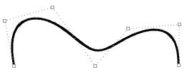
Curve degree is a whole positive number. Rhino allows working with any degree curve starting with 1. Degrees 1, 2, 3, and 5 are the most useful but the degrees 4 and those above 5 are not used much in the real world. Following are a few examples of curves and their degree:

Lines and polylines are degree-1 NURBS curves.

Circles and ellipses are examples of degree-2 NURBS curves.

Free-form curves are usually represented as degree-3 or 5 NURBS curves.

Control points

The control points of a NURBS curve is a list of at least (degree+1) points. The most intuitive way to change the shape of a NURBS curve is through moving its control points.

The number of control points that affect each span in a NURBS curve is defined by the degree of the curve. For example, each span in a degree 1 curve is affected only by the two end control points. In a degree 2 curve, three control points affect each span and so on.

Control points of degree-1 curves go through all curve control points. In a degree-1 NURBS curve, two (degree+1) control points define each span. Using five control points, the curve has four spans.

Circles and ellipses are examples of degree two curves. In a degree-2 NURBS curve, three (degree+1) control points define each span. Using five control points, the curve has three spans.

Control points of degree3 curves do not usually touch the curve, except at end points in open curves. In a degree3 NURBS curve, four (degree+1) control points define each span. Using five control points, the curve has two spans.

Weights of control points

Each control point has an associated number called weight. With a few exceptions, weights are positive numbers. When all control points have the same weight, usually 1, the curve is called non-rational. Intuitively, you can think of weights as the amount of gravity each control point has. The higher the relative weight a control point has, the closer the curve is pulled towards that control point.

It is worth noting that it is best to avoid changing curve weights. Changing weights rarely gives desired result while it introduces a lot of calculation challenges in operations such as intersections. The only good reason for using rational curves is to represent curves that cannot otherwise be drawn, such as circles and ellipses.

Figure 37: The effect of varying weights of control points on the result curve. The left curve is non-rational with uniform control point weights. The circle on the right is a rational curve with corner control points having weights less than 1.

Knots

Each NURBS curve has a list of numbers associated with it called a knots (sometimes referred to as knot vector). Knots are a little harder to understand and set. While using a 3-D modeler, you will not need to manually set the knots for each curve you create; a few things will be useful to learn about knots.

Knots are parameter values

Knots are a non-decreasing list of parameter values that lie within the curve domain. In Rhino, there is degree-1 more knots than control points. That is the number of knots equals the number of control points plus curve degree minus 1:

|knots| = |CVs| + Degree - 1

Usually, for non-periodic curves, the first degree many knots are equal to the domain minimum, and the last degree many knots are equal to the domain maximum.

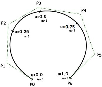
For example, the knots of an open degree-3 NURBS curve with 7 control points and a domain between 0 and 4 may look like <0, 0, 0, 1, 2, 3, 4, 4, 4>.

Figure 38: There are degree-1 more knots than control points. If the number of control points=7, and curve degree=3, then number of knots is 9. Knots values are parameters that evaluate to points on the 3D curve.

Scaling a knot list does not affect the 3D curve. If you change the domain of the curve in the above example from “0 to 4” to “0 to 1”, knot list get scaled, but the 3D curve does not change.

Figure 39: Scaling the knot list does not change the 3D curve.

We call a knot with value appearing only once as simple knot. Interior knots are typically simple as in the two examples above.

Knot multiplicity

The multiplicity of a knot is the number of times it is listed in the list of knots. The multiplicity of a knot cannot be more than the degree of the curve. Knot multiplicity is used to control continuity at the corresponding curve point.

Fully-multiple knots

A fully multiple knot has multiplicity equal to the curve degree. At a fully multiple knot there is a corresponding control point, and the curve goes through this point.

For example, clamped or open curves have knots with full multiplicity at the ends of the curve. This is why the end control points coincide with the curve end points. Interior fully multiple knots allow a kink in the curve at the corresponding point.

For example, the following two curves are both degree 3, and have the same number and location of control points. However they have different knots and their shape is also different. Fully multiplicity forces the curve through the associated control point.

Figure 40: (A) Clamped curves have fully-multiple knots at their start and end that is equal to the curve degree (3 in this case). The rest of the knots are simple. (B)' A fully multiple knot in the middle creates a kink and the curve is forced to go through the associated control point.

Uniform knots

A uniform list of knots in open curves satisfies the following condition:

Knots start with a fully-multiple knot, are followed by simple knots, and terminate with a fully-multiple knot. The values are increasing and equally spaced. This is typical of open (clamped ) curves. Periodic closed curves work differently as we will see later.

Figure 41: Uniform knot list means that spacing between knots is constant, with the exception of clamped curves where they can full multiplicity knot at start and end, and still be considered uniform. The left curve is periodic (closed without kink), and the right is clamped (open).

Non uniform knots

NURBS curves are allowed to have non-uniform spacing between knots. This can help control the curvature along the curve to create more smooth curves. Take the following example interpolating through points using non-uniform knots list in the left, and uniform in the right. In general, if a NURBS curve spacing of knots is proportional to the spacing between control points, then the curve is smoother.

Figure 42: Non-uniform knot list can help produce smoother curves. The curve on the left interpolate through points with non-uniform knots, and produces smoother curvature. The curve on the right interpolate through the same points but forces a uniform spacing of knots, resulting curve is not as smooth.

An example of a curve that is both non-uniform and rational is a NURBS circle. The following is a degree 2 curve with 9 control points and 10 knots. Domain is 0-4, and the spacing alternate between 0 and 1.

knots = <0,0,1,1,2,2,3,3,4,4> --- (full multiplicity in the interior knots)

spacing between knots = [0,1,0,1,0,1,0,1,0] --- (non-uniform)

Figure 43: A NURBS approximation of a circle is rational and non-uniform NURBS.

Evaluation rule

The evaluation rule uses a mathematical formula that takes a number within the curve domain and assigns a point. The formula takes into account the degree, control points, and knots.

Using this formula, specialized curve functions can take a curve parameter and produce the corresponding point on that curve. A parameter is a number that lies within the curve domain. Domains are usually increasing and consist of two numbers: the minimum domain parameter (usually referred to as t0) evaluates to the start point of the curve and the maximum parameter (t1) evaluates to the end point of the curve.

Figure 44: Evaluate parameters (a, b, c, …) to points on 3D curve (A, B, C, …). Minimum and maximum parameters (t0 and t1) evaluate to the start and end points of the 3D curve.

Characteristics of NURBS curves

In order to create a NURBS curve, you will need to provide the following information:

● Dimension, typically 3

● Degree, (sometimes use the order, which is equal to degree+1)

● Control points (list of points)

● Weight of the control point (list of numbers)

● Knots (list of numbers)

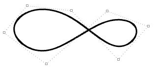
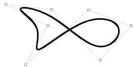
When you create a curve, you need to at least define the degree and locations of the control points. The rest of the information necessary to construct NURBS curves can be generated automatically. Selecting an end point to coincide with the start point would typically create a periodic smooth closed curve. The following table shows examples of open and closed curves:

Degree-1 open curve. The curve goes through all control points.

Degree-3 open curve. Both curve ends coincide with end control points.

Degree-3 closed periodic curve. The curve seam does not go through a control point.

Moving control points of a periodic curve does not affect curve smoothness.

Kinks are created when the curve is forced through some control points.

Moving the control points of a non-periodic curve does not guarantee smooth continuity of the curve, but enables more control over the outcome.

Clamped vs. periodic NURBS curves

The end points of closed clamped curves coincide with end control points. Periodic curves are smooth closed curves. The best way to understand the differences between the two is through comparing control points and knots.

The following is an example of an open, clamped non-rational NURBS curve. This curve has four control points, uniform knots with full-multiplicity at the start and end knots and the weights of all control points equal to 1.

Figure 45: Analyze degree-3 open non-rational NURBS curve.

The following circular curve is an example of a degree-3 closed periodic NURBS curve. It is also non-rational because all weights are equal. Note that periodic curves require more control points with few overlapping. Also the knots are simple.

Figure 46: Analyze degree-3 closed (periodic) NURBS curve.

Notice that the periodic curve turned the four input points into seven control points (degree+4), while the clamped curve used only the four control points. The knots of the periodic curve uses only simple knots, while the clamped curve start and end knots have full multiplicity forcing the curve to go through the start and end control points.

If we set the degree of the previous examples to 2 instead of 3, the knots become smaller, and the number of control points of periodic curves changes.

Figure 47: Analyze degree-2 open NURBS curve.

Figure 48: Analyze degree-2 closed (periodic) NURBS curve.

Weights

Weights of control points in a uniform NURBS curve are set to 1, but this number can vary in rational NURBS curves. The following example shows the effect of varying the weights of control points.

Figure 49: Analyze weights in open NURBS curve.

Figure 50: Analyze weights in closed NURBS curve.

Evaluating NURBS curves

Named after its inventor, Carl de Boor, the de Boor’s algorithm is a generalization of the de Casteljau algorithm for Bézier curves. It is numerically stable and is widely used to evaluate points on NURBS curves in 3-D applications. The following is an example for evaluating a point on a degree-3 NURBS curve using de Boor’s algorithm.

Input

Seven control points P₀ to P₆

Knots:

● u0 = 0.0

● u1 = 0.0

● u2 = 0.0

● u3 = 0.25

● u4 = 0.5

● u5 = 0.75

● u6 = 1.0

● u7 = 1.0

● u8 = 1.0

Output

Point on curve that is at u=0.4

Solution

1. Calculate coefficients for the first iteration:

Ac = (u – u₁) / ( u₁+₃ – u₁) = 0.8

Bc = (u – u₂) / ( u₂+₃ – u₂) = 0.53

Cc = (u – u₃) / ( u₃+₃ – u₃) = 0.2

2. Calculate points using coefficient data:

A = 0.2P₁ + 0.8P₂

B = 0.47 P₂ + 0.53 P₃

C = 0.8 P₃ + 0.2 P₄

3. Calculate coefficients for the second iteration:

Dc = (u – u₂) / (u₂+₃-₁ – u₂) = 0.8

Ec = (u – u₃) / (u₃+₃-₁ – u₃) = 0.3

4. Calculate points using coefficient data:

D = 0.2A+ 0.8B

E = 0.7B + 0.3C

5. Calculate the last coefficient:

Fc = (u – u₃)/ (u₃+₃-₂ – u₃) = 0.6

Find the point on curve at u=0.4 parameter:

F = 0.4D + 0.6E

Curve geometric continuity

Continuity is an important concept in 3D modeling. Continuity is important for achieving visual smoothness and for obtaining smooth light and airflow.

The following table shows various continuities and their definitions:

G0 (Position continuous)

Two curve segments joined together.

G1 (Tangent continuous)

Direction of tangent at joint point is the same for both curve segments.

G2 (Curvature Continuous)

Curvatures as well as tangents agree for both curve segments at the common endpoint.

GN

The curves agree to higher order.

Figure 51: Examining curve continuity with curvature graph analysis.

Curve curvature

Curvature is a widely used concept in modeling 3D curves and surfaces. Curvature is defined as the change in inclination of a tangent to a curve over unit length of arc. For a circle or sphere, it is the reciprocal of the radius and it is constant across the full domain.

At any point on a curve in the plane, the line best approximating the curve that passes through this point is the tangent line. We can also find the best approximating circle that passes through this point and is tangent to the curve. The reciprocal of the radius of this circle is the curvature of the curve at this point.

Figure 52: Examining curve curvature at different points.

The best approximating circle can lie either to the left or to the right of the curve. If we care about this, we establish a convention, such as giving the curvature positive sign if the circle lies to the left and negative sign if the circle lies to the right of the curve. This is known as signed curvature. Curvature values of joined curves indicate continuity between these curves.

Parametric surfaces

Surface parameters

A parametric surface is a function of two independent parameters (usually denoted u, v) over some two-dimensional domain. Take for example a plane. If we have a point P on the plane and two nonparallel vectors on the plane, a and b, then we can define a parametric equation of the plane in terms of the two parameters u and v as follows:

P = P’ + u * a + v * b

Where:

P’ is a known point on the plane

a is the first vector on the plane

b is the first vector on the plane

u is the first parameter

v is the first parameter

Figure 53: The parameter rectangle of a plane.

Another example is the sphere. The Cartesian equation of a sphere centered at the origin with radius R is

x² + y² + z² = R²

That means for each point, there are three variables (x, y, z), which is not useful to use for a parametric representation that requires only two variables. However, in the spherical coordinate system, each point is found using the three values:

r: radial distance between the point and the origin

θ: the angle from the x-axis in the xy-plane

ø: the angle from the z-axis and the point

Figure 54: Spherical coordinate system.

A conversion of points from spherical to Cartesian coordinate can be obtained as follows:

x = r * sin(ø) * cos(θ)

y = r * sin(ø) * sin(θ)

z = r * cos (ø)

Where:

r is distance from origin ≥ 0

θ is running from 0 to 2π

ø is running from 0 to π

Since r is constant in a sphere surface, we are left with only two variables, and hence we can use the above to create a parametric representation of a sphere surface:

u = θ

v = ø

So that:

x = r * sin(v) * cos(u)

y = r * sin(v) * sin(u)

z = r * cos(v)

Where (u, v) is within the domain (2 π, π)

Figure 55: The parameter rectangle of a sphere.

The parametric surface follows the general form:

x = x(u,v)

y = y(u,v)

z = z(u,v)

Where:

u and v are the two parameters within the surface domain or region.

Surface domain

A surface domain is defined as the range of (u,v) parameters that evaluate into a 3D point on that surface. The domain in each dimension (u or v) is usually described as two real numbers (u_min to u_max) and (v_min to v_max).

Changing a surface domain is referred to as reparameterizing the surface.

An increasing domain means that the minimum value of the domain points to the minimum point of the surface. Domains are typically increasing, but not always.

Figure 56: NURBS surface in 3-D modeling space (left). The surface parameter rectangle with domain spanning from u0 to u1 in the first direction and v0 to v1 in the second direction (right).

Surface evaluation

Evaluating a surface at a parameter that is within the surface domain results in a point that is on the surface. Keep in mind that the middle of the domain (midu, midv) might not necessarily evaluate to the middle point of the 3-D surface. Also, evaluating u- and v-values that are outside the surface domain will not give a useful result.

Figure 57: Surface evaluation.

Tangent plane of a surface

The tangent plane to a surface at a given point is the plane that touches the surface at that point. The z-direction of the tangent plane represents the normal direction of the surface at that point.

Figure 58: Tangent and normal vectors to a surface.

Surface geometric continuity

Many models cannot be constructed from one surface patch. Continuity between joined surface patches is important for visual smoothness, light reflection, and airflow.

The following table shows various continuities and their definitions:

G0 (Position continuous)

Two surfaces joined together.

G1 (Tangent continuous)

The corresponding tangents of the two surfaces along their joint edge are parallel in both u and v directions.

G2 (Curvature Continuous)

Curvatures as well as tangents agree for both surfaces at the common edge.

GN

The surfaces agree to higher order.

Figure 59: Examining surface continuity with zebra analysis.

Surface curvature

For surfaces, normal curvature is one generalization of curvature to surfaces. Given a point on the surface and a direction lying in the tangent plane of the surface at that point, the normal section curvature is computed by intersecting the surface with the plane spanned by the point, the normal to the surface at that point, and the direction. The normal section curvature is the signed curvature of this curve at the point of interest.

If we look at all directions in the tangent plane to the surface at our point, and we compute the normal curvature in all these directions, there will be a maximum value and a minimum value.

Figure 60: Normal curvatures.

Principal curvatures

The principal curvatures of a surface at a point are the minimum and maximum of the normal curvatures at that point. They measure the maximum and minimum bend amount of the surface at that point. The principal curvatures are used to compute the Gaussian and mean curvatures of the surface.

For example, in a cylindrical surface, there is no bend along the linear direction (curvature equals zero) while the maximum bend is when intersecting with a plane parallel to the end faces (curvature equals 1/radius). Those two extremes make the principal curvatures of that surface.

Figure 61: Principal curvatures at a surface point are the minimum and maximum curvatures at that point.

Gaussian curvature

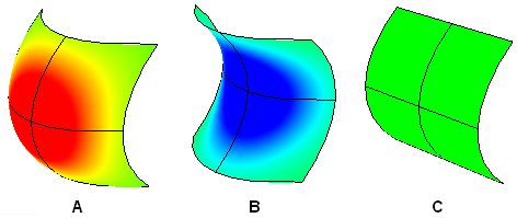
The Gaussian curvature of a surface at a point is the product of the principal curvatures at that point. The tangent plane of any point with positive Gaussian curvature touches the surface locally at a single point, whereas the tangent plane of any point with negative Gaussian curvature cuts the surface.

A: Positive curvature when surface is bowl-like. B: Negative curvature when surface is saddle-like. C: Zero curvature when surface is flat in at least one direction (plane, cylinder).


Figure 62: Analyzing the surface Gaussian curvature.

Mean curvature

The mean curvature of a surface at a point is one-half of the sums of the principal curvatures at that point. Any point with zero mean curvature has negative or zero Gaussian curvature.

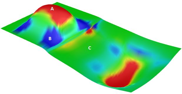
Surfaces with zero mean curvature everywhere are minimal surfaces. Physical processes which can be modeled by minimal surfaces include the formation of soap films spanning fixed objects, such as wire loops. A soap film is not distorted by air pressure (which is equal on both sides) and is free to minimize its area. This contrasts with a soap bubble, which encloses a fixed quantity of air and has unequal pressures on its inside and outside. Mean curvature is useful for finding areas of abrupt change in the surface curvature.

Surfaces with constant mean curvature everywhere are often referred to as constant mean curvature (CMC) surfaces. CMC surfaces include the formation of soap bubbles, both free and attached to objects. A soap bubble, unlike a simple soap film, encloses a volume and exists in equilibrium where slightly greater pressure inside the bubble is balanced by the area-minimizing forces of the bubble itself.

NURBS surfaces

You can think of NURBS surfaces as a grid of NURBS curves that go in two directions. The shape of a NURBS surface is defined by a number of control points and the degree of that surface in each one of the two directions (u- and v-directions). NURBS surfaces are efficient for storing and representing free-form surfaces with a high degree of accuracy. The mathematical equations and details of NURBS surfaces are beyond the scope of this text. We will only focus on the characteristics that are most useful for designers.

Figure 63: NURBS surface with red isocurves in the u-direction and green isocurves in the v-direction.

Figure 64: The control structure of a NURBS surface.

Figure 65: The parameter rectangle of a NURBS surface.

Evaluating parameters at equal intervals in the 2-D parameter rectangle does not translate into equal intervals in 3-D space in most cases.

Figure 66: Evaluating surfaces.

Characteristics of NURBS surfaces

NURBS surface characteristics are very similar to NURBS curves except there is one additional parameter. NURBS surfaces hold the following information:

● Dimension, typically 3

● Degree in u and v directions: (sometimes use order which is degree + 1)

● Control points (points)

● Weights of control points (numbers)

● Knots (numbers)

As with the NURBS curves, you will probably not need to know the details of how to create a NURBS surface, since 3-D modelers will typically provide good set of tools for this. You can always rebuild surfaces (and curves for that matter) to a new degree and number of control points. Surface can be open, closed, or periodic. Here are few examples of surfaces:

Degree-1 surface in both u- and v-directions.

All control points lie on the surface.

Degree-3 in the u-direction and degree1 in the v-direction open surface.

The surface corners coincide with corner control points.

Degree-3 in the u-direction and degree 1 in the v-direction closed (non-periodic) surface.

Some control points coincide with the surface seam.

Moving control points of a closed (non-periodic) surface causes a kink and the surface does not look smooth.

Degree 3 the u-direction and degree 1 in the v-direction periodic surface.

The surface control points do not coincide with the surface seam.

Moving the control points of a periodic surface does not affect surface smoothness or create kinks.

Singularity in NURBS surfaces

For example, if you have a linear edge of a simple plane, and you drag the two end control points of an edge so they overlap (collapse) at the middle, you will get a singular edge. You will notice that the surface isocurves converge at the singular point.

Figure 67: Collapse two corner points of a rectangular NURBS surface to create a triangular surface with singularity. The parameter rectangle remains rectangular.

The above triangular shape can be created without singularity. You can trim a surface with a triangle polyline. When you examine the underlying NURBS structure, you see that it remains a rectangular shape.

Figure 68: Trim a rectangular NURBS surface to create a trimmed triangular surface.

Other common examples of surfaces that are hard to generate without singularity are the cone and the sphere. The top of a cone and top and bottom edges of a sphere are collapsed into one point. Whether there is singularity or not, the parameter rectangle maintains a more or less rectangular region.

Trimmed NURBS surfaces

NURBS surfaces can be trimmed or untrimmed. Trimmed surfaces use an underlying NURBS surface and closed curves to trim out part of that surface. Each surface has one closed curve that defines the outer border (outer loop) and can have non-intersecting closed inner curves to define holes (inner loops). A surface with an outer loop that is the same as that of its underlying NURBS surface and that has no holes is what we refer to as an untrimmed surface.

Figure 69: Trimmed surface in modeling space (left) and in parameter rectangle (right).

Polysurfaces

A polysurface consists of two or more (possibly trimmed) NURBS surfaces joined together. Each surface has its own structure, parameterization, and isocurve directions that do not have to match. Polysurfaces are represented using the boundary representation (BRep). The BRep structure describes surfaces, edges, and vertices with trimming data and connectivity among different parts. Trimmed surface are also represented using BRep data structure.

Figure 70: Polysurfaces are made out of joined surfaces with common edges aligning perfectly within tolerance.

The BRep is a data structure that describes each face in terms of its underlying surface, surrounding 3-D edges, vertices, parameter space 2-D trims, and relationship between neighboring faces. BRep objects are also called solids when they are closed (watertight).

An example polysurface is a simple box that is made out of six untrimmed surfaces joined together.

Figure 71: Box made out of six untrimmed surfaces joined in one polysurface.

The same box can be made using trimmed surfaces, such as the top one in the following example.

Figure 72: Box faces can be trimmed.

The top and bottom faces of the cylinder in the following example are trimmed from planar surfaces.

Figure 73: The control points of the underlying surfaces.

We saw that editing NURBS curves and untrimmed surfaces is intuitive and can be done interactively by moving control points. However, editing trimmed surfaces and polysurfaces can be challenging. The main challenge is to be able to maintain joined edges of different faces within the desired tolerance. Neighboring faces that share common edges can be trimmed and do not usually have matching NURBS structure, and therefore modifying the object in a way that deforms that common edge might result in a gap.

Figure 74: Two triangular faces joined in one polysurface but do not have matching joined edge. Moving one corner create a hole.

Another challenge is that there is typically less control over the outcome, especially when modifying trimmed geometry.

Figure 75: Once a trimmed surface is created, there is limited control to edit the result.

Figure 76: Use cage edit technique in Rhino to edit polysurfaces.

Trimmed surfaces are described in parameter space using the untrimmed underlying surface combined with the 2-D trim curves that evaluate to the 3-D edges within the 3-D surface.

Tutorials

The following tutorials use the concepts learned in this chapter. They use Rhinoceros 5 and Grasshopper 0.9.

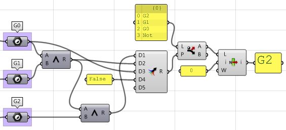
Continuity between curves

Examine the continuity between two input curves. Continuity assumes that the curves meet at the end of the first curve and the start of the second curve.

Input

Two input curves.

Parameters

Calculate the following to be able to decide the continuity between two curves:

● The end point of the first curve (P1)

● The start point of the second curve (P2)

● The tangent at the end of the first curve and at the start of the second curve (T1 and T2).

● The curvature at the end of the first curve and at the start of the second curve (C1 and C2).

Solution

1. Reparameterize the input curves. We do that so that we know that the start of the curve evaluates at t=0 and the end at t=1.

2. Extract the end and start points of the two curves, and check whether they coincide. If they do, the two curves are at least G0 continuous.

3. Calculate tangents.

4. Compare the tangents using the dot product. Make sure to unitize vectors. If the curves are parallel, then we have at least G1 continuity.

5. Calculate curvature vectors.

6. Compare curvature vectors, and if they agree, the two curves are G2 continuous.

7. Create logic that filters through the three results (G1, G2, and G3) and select the highest continuity.

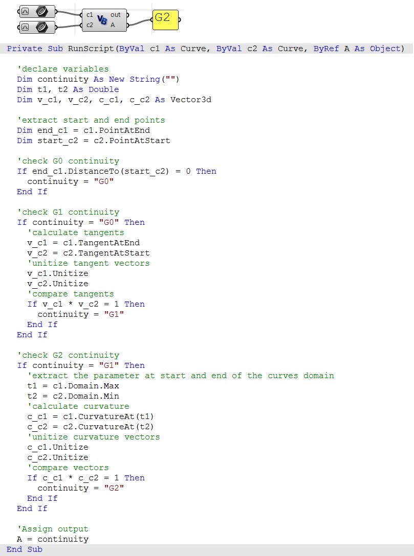
Using the Grasshopper VBScript component

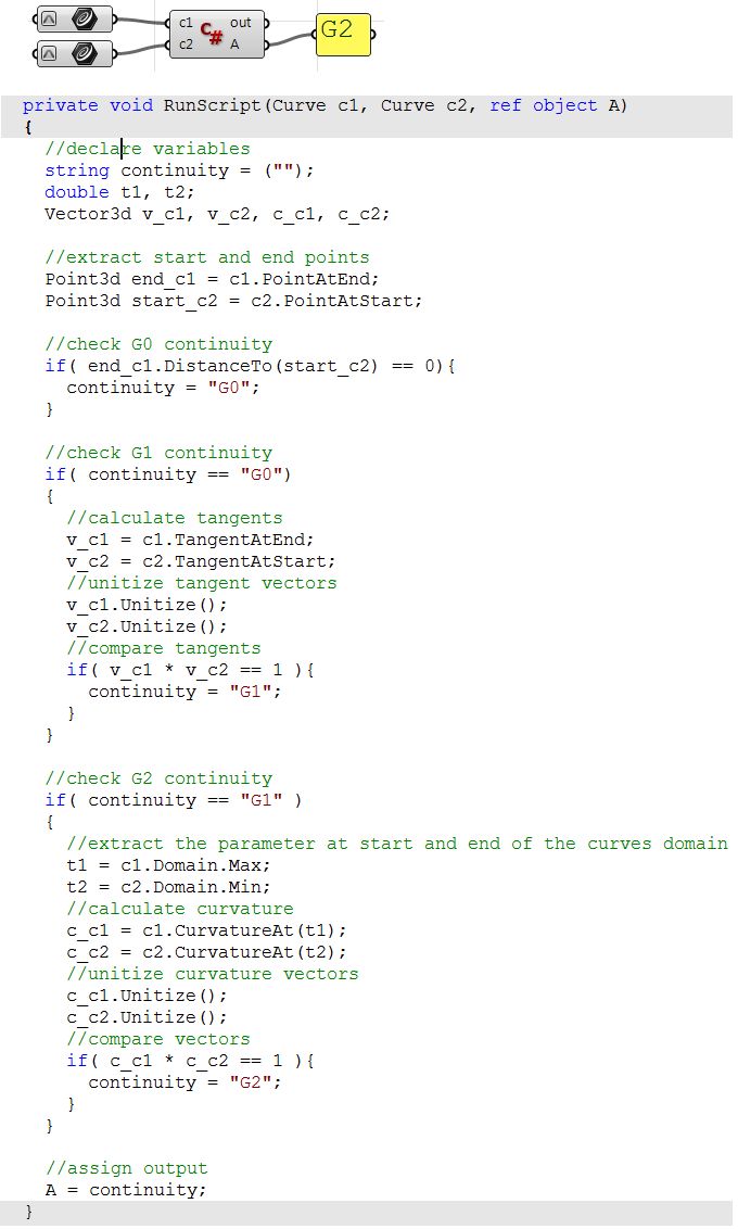
Using the Grasshopper C# component

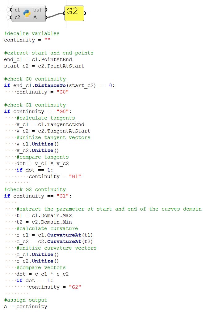
Using the Grasshopper Python component

Surfaces with singularity

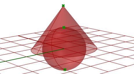
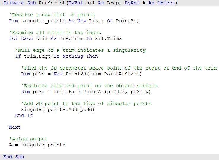
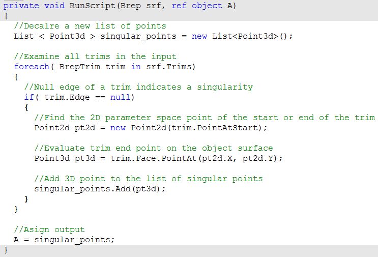
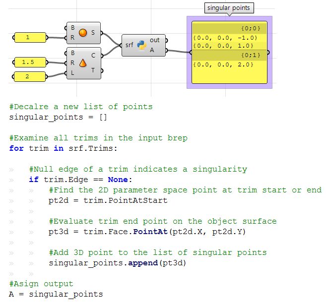
Extract singular points in a sphere and a cone.

Input

One sphere and one cone.

Parameters

Singularity can be detected through analyzing the 2-D parameter space trims that have invalid or zero-length corresponding edges. Those trims ought to be singular.

Solution

1. Traverse through all trims in the input.
2. Check if any trim has an invalid edge and flag it as a singular trim.
3. Extract point locations in 3-D space.

Using the Grasshopper VBScript component

Using the Grasshopper C# component

Using the Grasshopper Python component

References

Edward Angel, "Interactive Computer Graphics with OpenGL,” Addison Wesley Longman, Inc., 2000.

James D Foley, Steven K Feiner, John F Hughes, "Introduction to Computer Graphics" Addison-Wesley Publishing Company, Inc., 1997.

James Stewart, "Calculus," Wadsworth, Inc., 1991.

Kenneth Hoffman, Ray Kunze, “Linear Algebra”, Prentice-Hall, Inc., 1971

Rhinoceros® help document, Robert McNeel and Associates, 2009.

Essential Mathematics for Computational Design

Contents

Vector Mathematics

Vector representation

Position vector

Vectors vs. points

Vector length

Unit vector

Vector operations

Vector scalar operation

Vector addition

Vector subtraction

Vector properties

Vector dot product

Vector dot product, lengths, and angles

Dot product properties

Vector cross product

Cross product and angle between vectors

Cross product properties

Vector equation of line

Vector equation of a plane

Tutorials

Face direction

Exploded box

Tangent spheres

Matrices and Transformations

Matrix operations

Matrix multiplication

Identity matrix

Transformation operations

Translation (move) transformation

Rotation transformation

Scale transformation

Shear transformation

Mirror or reflection transformation

Planar Projection transformation

Tutorial

Multiple transformations

Parametric Curves and Surfaces

Parametric curves

Curve parameter

Curve domain or interval

Curve evaluation

Tangent vector to a curve

Cubic polynomial curves

Evaluating cubic Bézier curves

NURBS curves

Degree

Control points

Weights of control points

Knots

Knots are parameter values

Knot multiplicity

Fully-multiple knots

Uniform knots

Non uniform knots

Evaluation rule

Characteristics of NURBS curves

Clamped vs. periodic NURBS curves

Weights

Evaluating NURBS curves

Curve geometric continuity

Curve curvature

Parametric surfaces

Surface parameters

Surface domain

Surface evaluation

Tangent plane of a surface

Surface geometric continuity

Surface curvature

Principal curvatures

Gaussian curvature

Mean curvature

NURBS surfaces

Characteristics of NURBS surfaces

Singularity in NURBS surfaces

Trimmed NURBS surfaces

Polysurfaces

Tutorials

Continuity between curves