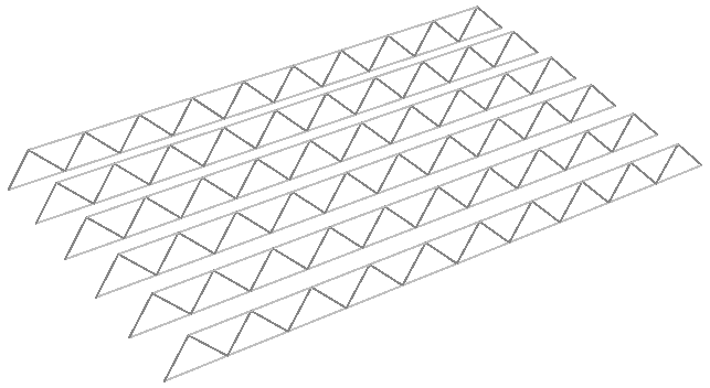
Essential Algorithms and Data Structures for Computational Design
The Essential Algorithms and Data Structures for Computational Design, by Rajaa Issa, introduces effective methodologies to develop complex 3D modeling algorithms using Grasshopper. It also covers extensively the data structure adopted by Grasshopper and its core organization and management tools.
The full contents of the book are produced here with the authorization of the authors and are directed towards designers who are interested in parametric design and have little or no background in programming. All concepts are explained visually using Grasshopper® (GH), the generative modeling environment for Rhinoceros® (Rhino). This book is not intended as a beginner's guide to Grasshopper in terms of user interface or tools. Basic knowledge of the interface and workflow is assumed. For more resources and getting started guides, go to the learn section in [rhino3d.com]. The content is divided into three chapters. Chapter 1 discusses algorithms and data. It introduces a methodology to help create and manage parametric solutions. It also introduces basic data concepts such as data types, sources and common ways to process them. Chapter 2 reviews basic data structures in Grasshopper. That includes single items and lists. Chapter 3 includes an in-depth review of the tree data structure in Grasshopper and practical applications in design problems. All Grasshopper examples and tutorials are written with Rhinoceros version 6 and are included in the download.
Contents
- 1 Chapter 1: Algorithms and Data
- 2 Chapter Two: Introduction to Data Structures
- 3 Chapter Three: Advanced Data Structures
- 3.1 The Grasshopper data structure
- 3.2 Generating trees
- 3.3 Tree matching
- 3.4 Traversing trees
- 3.5 Basic tree operations
- 3.5.1 Viewing the tree structure
- 3.5.2 List operations on trees
- 3.5.3 Grafting from lists to a trees
- 3.5.4 Flattening from trees to lists
- 3.5.5 Combining data streams
- 3.5.6 Flipping the data structure
- 3.5.7 Simplifying the data structure
- 3.5.8 Basic tree operations tutorial #1
- 3.5.9 Simple tree operations tutorial #2
- 3.6 Advanced tree operations
- 3.7 Advanced data structures tutorials
Chapter 1: Algorithms and Data
Algorithms and data are the two essential parts of any parametric design solution, but writing algorithms is not trivial and requires a skill that does not come easy to intuitive designers. The algorithmic design process is highly logical and requires an explicit statement of the design intention and the steps to achieve them. This chapter introduces a methodology to help creative designers develop new algorithmic solutions. All algorithms involve manipulating data and hence Algorithms and Data are tightly connected. We will introduce the basic concepts of data types and processes.
Algorithmic design
We can define algorithmic design as a design method where the output is achieved through well-defined steps. In that sense, many human activities are algorithmic. Take, for example, baking a cake. You get the cake (output) by using a recipe (well-defined steps). Any change in the ingredients (input) or the baking process results in a different cake. We will analyze the parts of typical algorithms, and identify a strategy to build algorithmic solutions from scratch. Regardless of its complexity, all algorithmic solutions have 3 building blocks: input, key process, and output. Note that the key process may require additional input and processes.
Throughout this text, we will organize and label the solutions to identify the three blocks clearly. We will also use consistent color coding to visually distinguish between the parts. This will help us become more comfortable with reading algorithms and quickly identify input, key processing steps, and properly collect and display output. Visual cues are important to develop fluency in algorithmic thinking.
In general, reading existing algorithmic solutions is relatively easy, but building new ones from scratch is much harder and requires a new set of skills. While it is useful to know how to read and modify existing solutions, it is essential to develop algorithmic design skills to build new solutions from scratch.
Algorithms parts
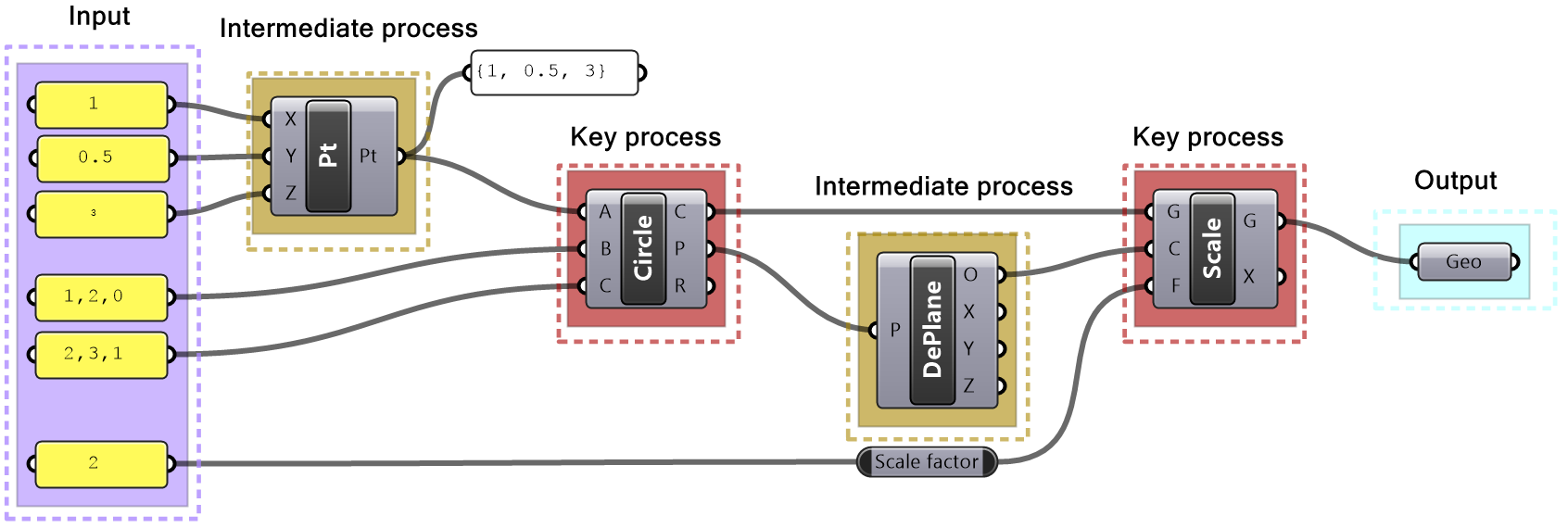
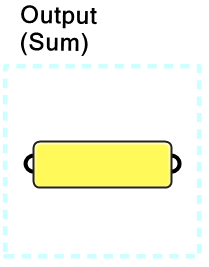
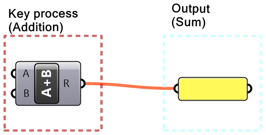
In Grasshopper, a solution flows from left to right. At the far left are input values and parameters, and the far-right has the output. In between are one or more key processes, and sometimes additional input and output. Let’s take a simple example to help identify the three parts of any algorithm (input, key process, output). The simple addition algorithm includes two numbers (input), the sum (output) and one key process that takes the numbers and gives the result. We will use purple for the input, maroon for the key processes and light blue for the output. We will also group and label the different parts and adhere to organizing the Grasshopper solutions from left to right.
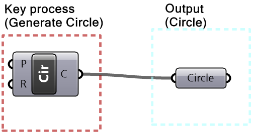
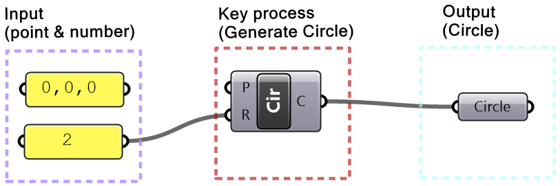
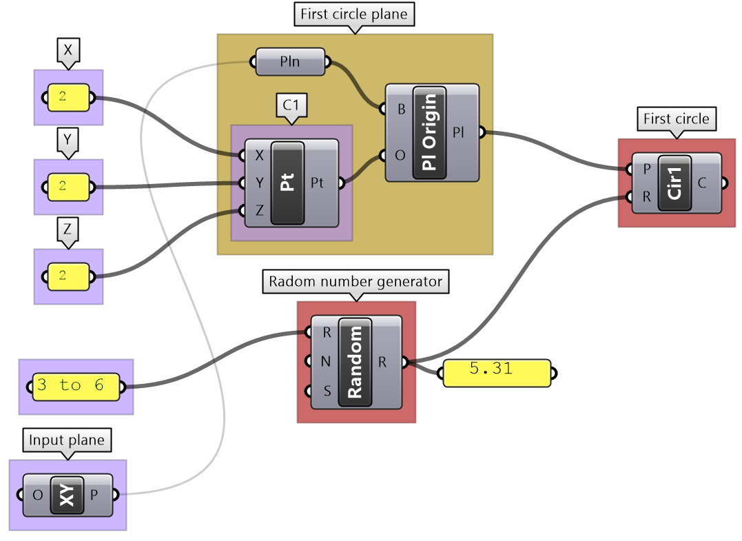
Algorithms may involve intermediate processes. For example, suppose we need to create a circle (output) using a center and a radius (input). Notice that the input is not sufficient because we do not know the plane on which the circle should be created. In this case, we need to generate additional information, namely the plane of the circle. We will call this an intermediate process and use brown color to label it.
Some solutions are not written with styles and hence are hard to read and build on. It is very important that you take the time to organize and label your solutions to make it easier to understand, debug and use by others.
Solution
In order to figure out what the algorithm is meant to do, we need to group the input on the left side, and collect the output on the right side, then organize the processes in the order or execution. We then step through the solution from left to right to deduce what it does. We can examine and preview the output in each step.
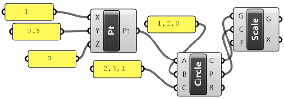
The example of the tutorial is meant to create a circle that is twice as large as another circle that goes through three given points. One of the points is constructed out of its 3 coordinates.
Designing algorithms: the 4-step process
Before we generalize a method to design algorithms, let’s examine an algorithm we commonly use in real life such as baking a cake. If you already have a recipe for a cake, you simply get the recommended ingredients, mix them, pour in a pan, put in preheated oven for a certain amount of time, then serve. If the recipe is well documented, then it is relatively straightforward to use.
As you become more proficient in baking cakes, you may start to modify the recipe. Perhaps add new ingredients (chocolate or nuts) or use different tools (cupcake container).
When designers write algorithms, they typically try to search for existing solutions and modify to fit their purposes. While this is a good entry point, using existing solutions can be frustrating and timeconsuming.
Also, existing solutions have their own flavor and that may influence design decisions and limit creativity. If designers have unique problems, and they often do, they have no choice but to create new solutions from scratch; albeit a much harder endeavor.
Back to our example, the task of baking a cake is much harder if you don’t have a recipe to follow and have not baked one before. You will have to guess the ingredients and the process. You will likely end up with bad results in the first few attempts, until you figure it out! In general, when you create a new recipe, you have to follow the process in reverse. You start with an image of the desired cake, you then guess the ingredients, tools and steps. Your thinking goes along the following lines:
- The cake needs to be baked, so I need an oven and time;
- What goes in the oven is a cake batter held by a container;
- The batter is a mix of ingredients;
We can use a similar methodology to design parametric algorithm from scratch. Keep in mind that creating new algorithms is a “skill” and it requires patience, practice and time to develop.
Algorithmic thinking in 3D modeling vs parametric design
3D modeling involves certain level of algorithmic thinking, but it has many implicit steps and data. For example, designing a mass model using a 3D modeler may involve the following steps:
- 1- Think about the output (e.g. a mass out of few intersecting boxes)
- 2- Identify a command or series of commands to achieve the output ( e.g. run Box command few times, Move, Scale or Rotate one or more boxes, then BooleanUnion the geometry).
At that point, you are done!
Data such as the base point for your initial box, width, height, scale factor, move direction, rotation angle, etc. are requested by the commands, and the designer does not need to prepare ahead of time. Also, the final output (the boolean mass) becomes directly available and visible as an object in your document.
Algorithmic solutions are not interactive and require explicit articulation of data and processes. In the box example, you need to define the box orientation and dimensions. When copy, you need a vector and when rotate you need to define the plane and angle or rotation.
Designing algorithms
Designing algorithms requires knowledge in geometry, mathematics and programming. Knowledge in geometry and mathematics is covered in the Essential Mathematics for Computational Design. As for programming skills, it takes time and practice to build the ability to formulate design intentions into logical steps to process and manage geometric data. To help get started, it is useful to think of any algorithm as a 4-step process as in the following:
| 1- Clearly identify the desired outcome | Output |
| 2- Identify key steps to reach the outcome | Key processes |
| 3- Examine initial data and parameters | Input |
| 4- Define intermediate steps to generate missing data | Intermediate input + processes |
Thinking in terms of these 4 steps is key to developing the skill of algorithmic design. We will start with simple examples to illustrate the methodology, and gradually apply on more complex examples.
| Step 1: Output: The sum of the 2 numbers. Use a Panel to collect the sum. | |
| Step 2: Key process: Addition. Use the Addition component that takes 2 numbers and gives the sum. | |
| Step 3: Input: 2 numbers. Use a Panel to hold the values of input numbers. |
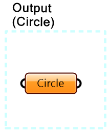
| Step 1: Output: Circle. Use the Circle parameter to collect the output. | |
| Step 2: Key process: Identify a key process that generates a circle from a radius. Use the Circle component in Grasshopper. | |
| Step 3: Input: Use the given input (center and radius). Feed the radius to the Circle component. | |
| Step 4: Intermediate process: The circle needs the center, and also the plane on which the circle is located. Assume the circle is on a plane parallel to the XY-Plane and use the circle center as the origin of the plane. |
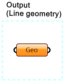
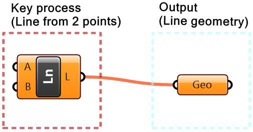
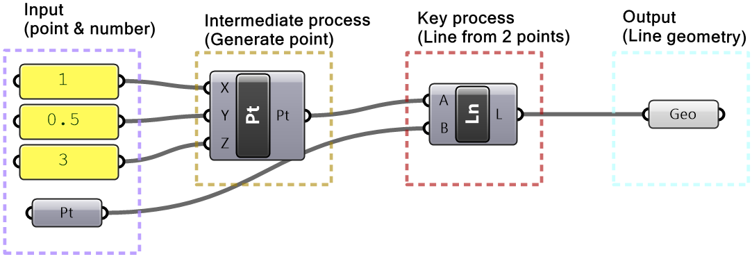
| Step 1: Output: The line geometry. Use the Geometry parameter to collect the output. | |
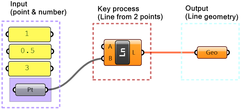
| Step 2: Key process: Identify a key process that generates a line from 2 points. Use the Line component in Grasshopper. | |
| Step 3: Input: Use the given input (referenced point and 3 coordinates). Feed one point to one of the ends of the line. | |
| Step 4: Intermediate process: Before we can use the coordinates as a point, we need to construct a point. |
Data
Data is information stored in a computer and processed by a program. Data can be collected from different sources, it has many types and is stored in well-defined structures so that it can be used efficiently. While there are commonalities when it comes to data across all scripting languages, there are also some differences. This book explores data and data structures specific to Grasshopper.
Data sources
In Grasshopper, there are three main ways to supply data to processes (or what is called components): internal, referenced and external.
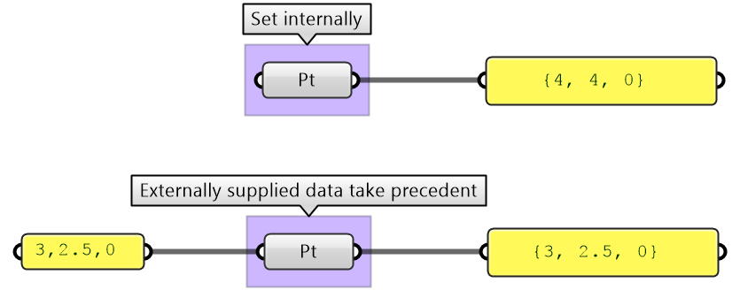
| 1- Internally set data: Data can be set inside any instance of a parameter. Once set, it remains constant, unless manually changed or overridden by external input. This is a good way when you do not generally need to change the data after it is set (constant). Data is stored inside the GH file. | |
| 2- Referenced data: Data can be referenced from Rhino or some external document. For example, you can reference a point created in a Rhino document. When you move the point in Rhino, its reference in Grasshopper updates as well. Grasshopper files are saved separately from Rhino files, and hence if the GH file has referenced data, the Rhino file needs to be saved and passed along with the GH file to avoid any loss of data. | |
| 3- Externally supplied data: Data can be supplied from previous processes. This method is best suited for dynamic data or data controlled parametrically. Externally supplied data to a parameter takes precedent over the internal or referenced values (when both exist). |
Data types
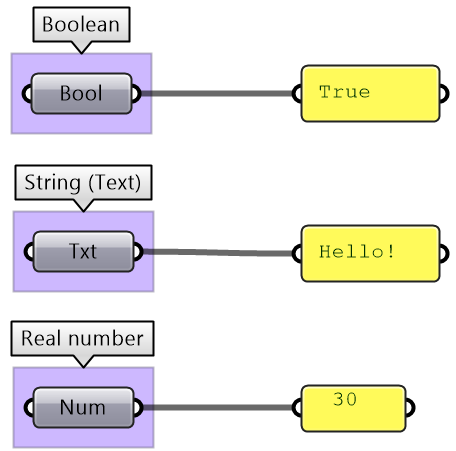
All programming languages identify the kind of data used in terms of the values that can be assigned to and the operations and processes it can participate in. There are common data types such as Integer, Number, Text, Bool (true or false), and others. Grasshopper lists those under the Params > Primitives tab.
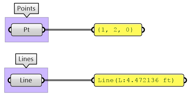
Grasshopper supports geometry types that are useful in the context of 3D modeling such as Point (3 numbers for coordinates), Line (2 points), NURBS Curve, NURBS Surface, Brep, and others. All geometry types are included under the Param> Geometry tab in GH.
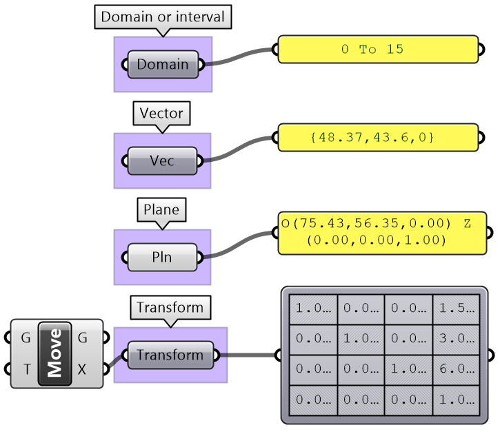
There are other mathematics types that designers do not usually use in 3D modeling, but are very common in a parametric design such as Domains, Vectors, Planes, and Transformation Matrices. GH provides a rich set of tools to help create, analyze and use these types. To fully understand the mathematical as well as geometry types such as NURBS curves and surfaces, you can refer to the Essential Mathematics for Computational Design book by the author.
The parameters in GH can be used to convert data from one type to another (cast). For example, if you need to turn a text into a number, you can feed your text into a Number parameter. If the text cannot be converted, you’ll get an error.
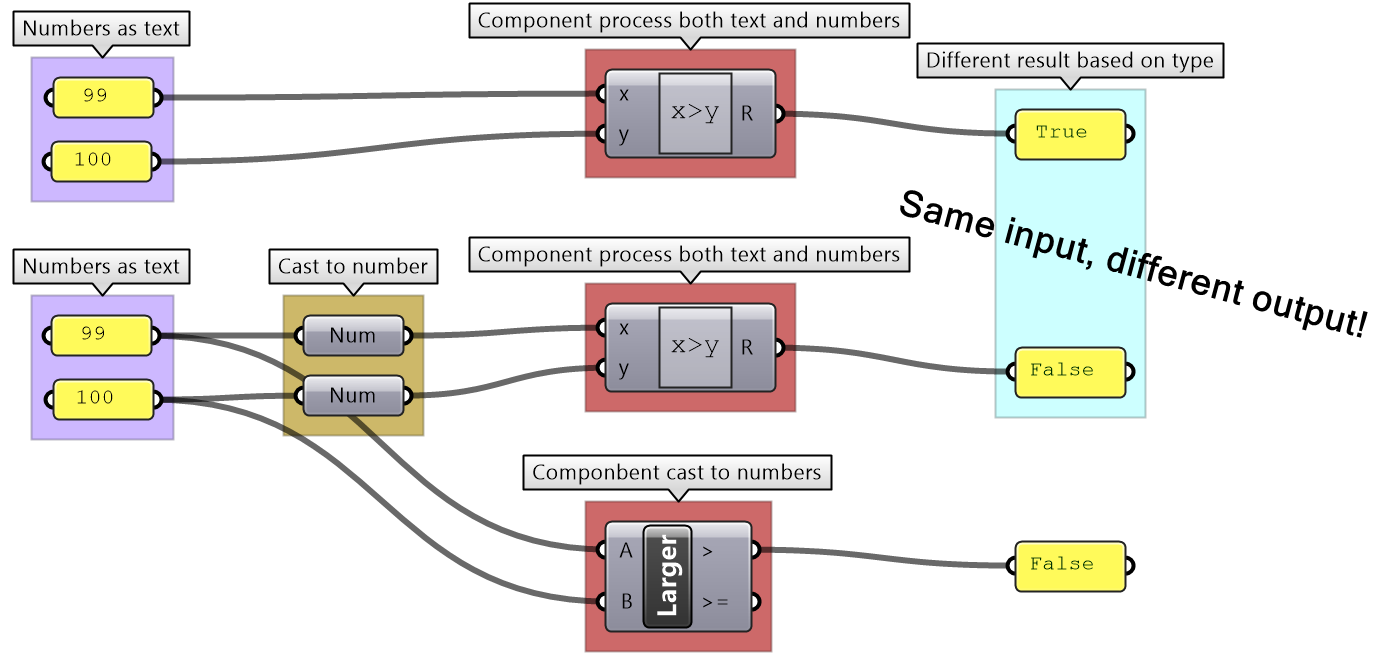
Grasshopper components internally convert the input to suitable types when possible. For example, if you feed a “text” to the Addition component, GH tries to read the text as a number. If a component can process more than one type, it uses the input type without conversion. For example, equality in an expression can compare text as well as numbers. In such a case, make sure you use the intended type to avoid confusion.
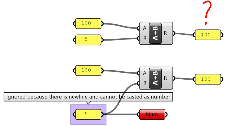
It is worth noting that sometimes GH components simply ignore invalid input (null or wrong type). In such cases, you are likely to end up with an unexpected result and hard to find the bug. It is very important to verify the output from each component before using it.
Processing data
Algorithmic designs use many data operations and processes. In the context of this book, we will focus on five categories: numeric and logical operations, analysis, sorting, and selection.
Numeric operations
Numeric operations include operations such as arithmetic, trigonometry, polynomials, and complex numbers. GH has a rich set of numeric operations, and they are mostly found under the Math tab.
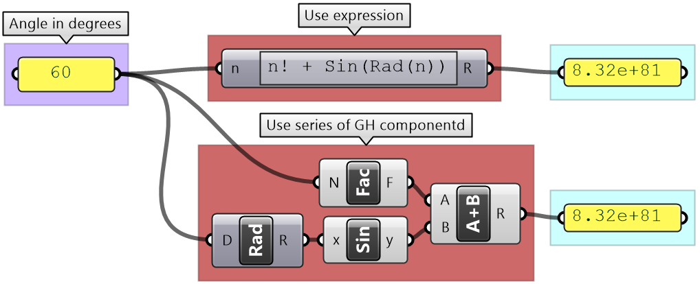
There are two main ways to perform operations in GH. First by using designated components for specific operations such as Addition, Subtraction, and Multiplication.
Second, use an Expression component where you can combine multiple operations and perform a rich set of math and trigonometry operations, all in one expression.
The Expression component is more robust and readable when you have multiple operations.
Input to Expressions can be treated as text depending on the context.
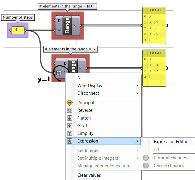
It is worth mentioning that most numeric input to components allow writing an expression to modify the input inline. For example, the Range component has N (number of steps) input. If you right-mouse click on “N”, you can set an expression. You always use “x” to represent the supplied input regardless of the name.
Logical operations
Main logical operations in GH include equalities, sets and logical operations.
Logical operations are used to create conditional flows of data. For example, if you like to draw a sphere only when the radius is between two values, then you need to create a logic that blocks the radius when it is not within your limits.
Data analysis
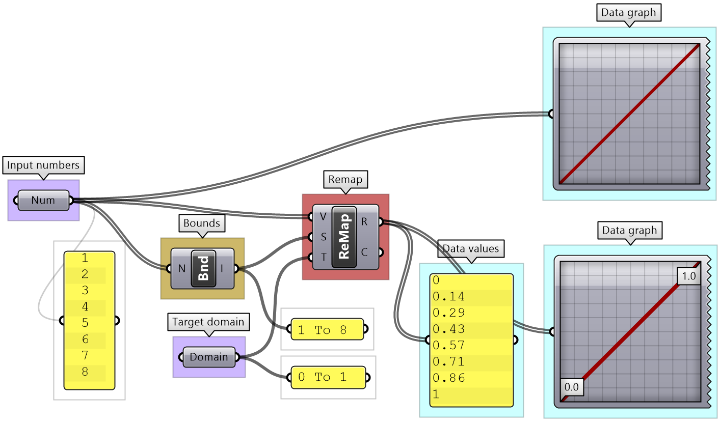
There are many tools in GH to examine and preview data. Panel is used to show the full details of the data and its structure, while the Parameter Viewer shows the data structure only. Other analysis components include Quick Graph that plots data in a graph, and Bounds to find the limits in a given set of numbers (the min and max values in the set).
Sorting
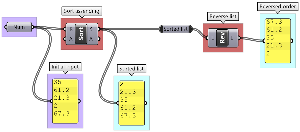
GH has designated components to sort numeric and geometry data. The Sort List component can sort a list of numeric keys. It can sort a list of numbers in ascending order or reverse the order. You can also use the Sort List component to sort geometry by some numeric keys, for example sort curves by length. GH has components designated to sort geometry sets such as Sort Points to sort points by their coordinates.
Selection
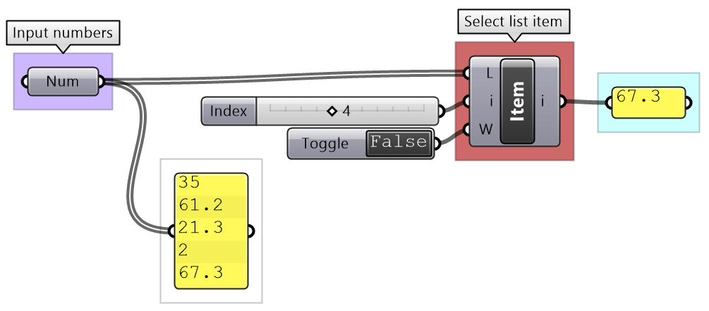
3D modeling allows picking specific or a group of objects interactively, but this is not possible in algorithmic design. Data is selected in GH based on the location within the data structure, or by a selection pattern. For example, the List Item component allows selecting elements based on their indices.
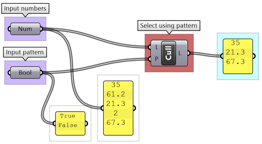
The Cull Pattern component allows using some repeated pattern to select a subset of the data.
As you can see from the examples, selecting specific items or using cull components yield a subset of the data, and the rest is thrown away. Many times you only need to isolate a subset to operate on, then recombine back with the original set. This is possible in GH, but involves more advanced operations. We will get into the details of these operations when we talk about advanced data structures in Chapter 3.
Mapping
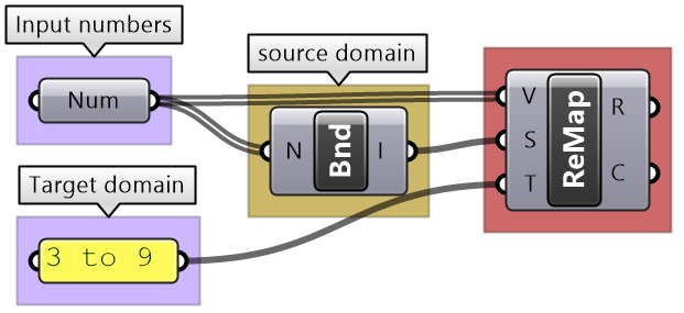
That refers to the linear mapping of a range of numbers where each number in a set is mapped to exactly one value in the new set. GH has a component to perform linear mapping called ReMap. You can use it to scale a set of numbers from its original range to a new one. This is useful to scale your range to a domain that suits your algorithm’s needs and limitations.
Converting data involves mapping. For example, you may need to convert an angle unit from degrees to radians ( GH components accept angles in radians only).
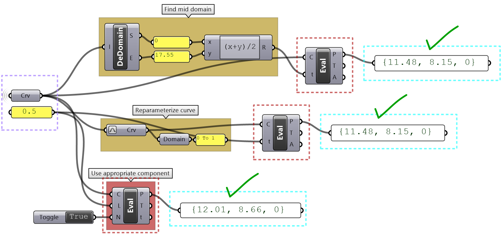
As you know, parametric curves have “domains” (the range of parameters that evaluate to points on the curve). For example, if the domain of a given curve is between 12.5 to 51.3, evaluating the curve at 12.5 gives the point at the start of the curve. Many times you need to evaluate multiple curves using consistent parameters. Reparameterizing the domain of curves to some unified range helps solve this problem. One common domain to use is “0 To 1”. At the input of each curve in any GH component, there is the option to Reparameterize which resets the domain of the curve to be “0 to 1”.
Flow control tutorial
What is the purpose of the following algorithm? Notate and color code to describe the purpose of each part.
| Analyze the algorithm |
| The algorithm has an output that is a sphere, a radius input and some conditional logic to process the radius. |
| Notate and color-code the solution |
| From testing the output and following the steps of the solution it becomes apparent that the intention is to make sure that the radius of the sphere cannot be less than 1 unit. |
| Test with radius < 1 |
Data processing tutorial
Given a list of point coordinates, do the following:
- 1- Analyze the list to understand the data.
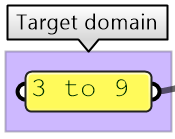
- 3- Write an algorithm to use the input to construct a list of type Point with coordinates mapped to a domain between 3 and 9.
Note that the input list is organized so that the first 3 numbers refer to the x,y,z of the first point, the second 3 numbers belong to the second point and so on.
| Analyze the algorithm | |
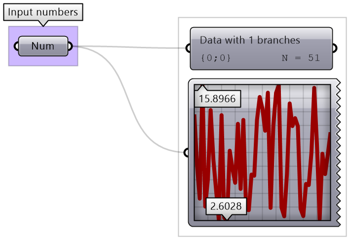
| There is a list of 51 numbers (3 coordinates for each point implies the list includes 17 points) Using a QuickGraph, we can see that the range of values are between 2.60 and 15.89. We can also see that the values are distributed randomly. One other input is the target domain: | |
| Use the 4-step process to solve the algorithms | |
| Output: List of points. | |
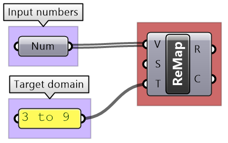
| Key Process #1 Remap Coordinates: Map the coordinates list from its current domain to a new domain 3 to 9 Use ReMap component. | |
| Intermediate processes #1 The input domain is missing and can be extracted using Bounds component | |
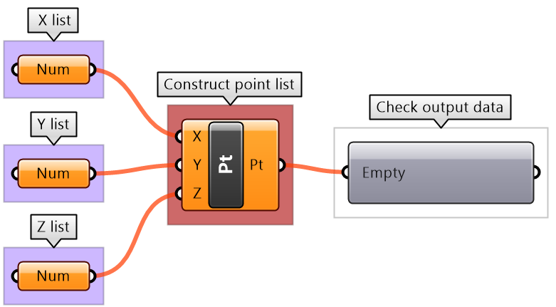
| Key Process #2 Construct Points: Construct points from coordinates. Use Construct Point (Pt) component | |
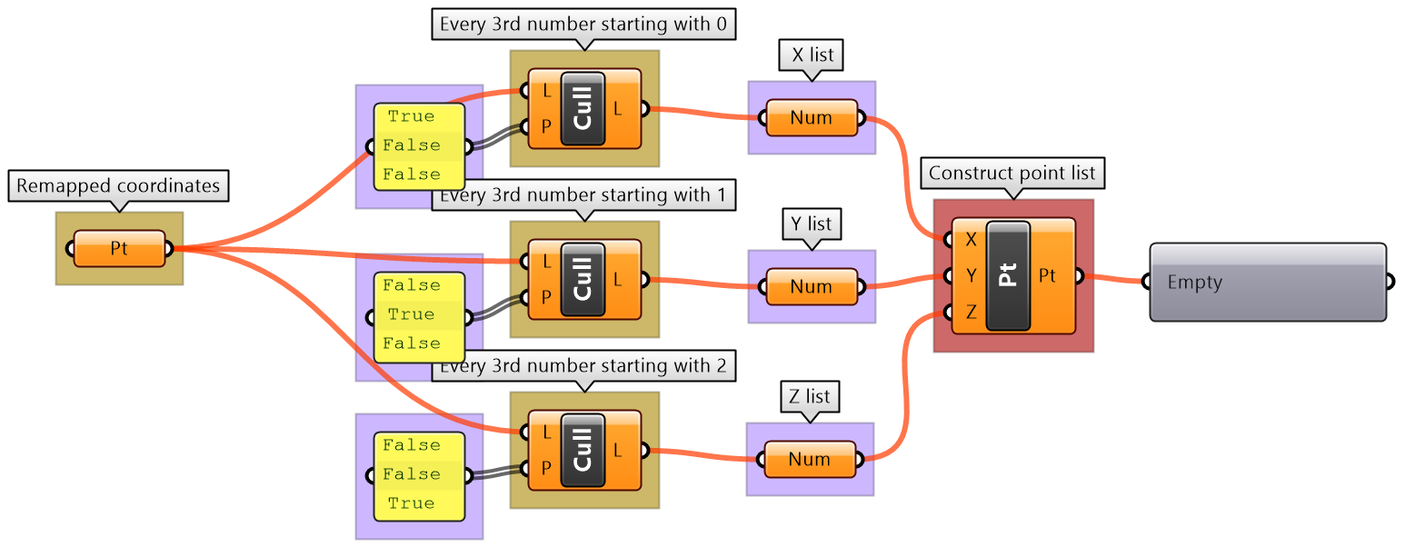
| Intermediate processes #2 Extract all X coordinates as one list, Y in another and Z in the third. Use Cull Pattern component with appropriate pattern to extract each coordinate as a separate list. The input to Cull is the remapped points from process #1 | |
| Putting it all together | |
Pitfalls of algorithmic design
Writing elegant algorithms that are efficient and easy to read and debug is hard. We explained in this chapter how to write algorithms with style using color-coding and labeling. We also articulated a 4-step process to help develop algorithms. Following these guides help minimize bugs and improve the readability of the scripts. We will list a few of the common issues that lead to an incorrect or unintended result.
Invalid or wrong type input
If the input is of the wrong type or is invalid, GH changes the color of components to red or orange to indicate an error warning, with feedback about what the issue might be. This is helpful, but sometimes faulty input goes unnoticed if the components assign a default value, or calculate an alternative value to replace the input, that is not what was intended. It is a good practice to always double-check the input (hook to a panel or parameter viewer and label the input). To avoid using the wrong types, it is advisable to convert to the intended type to ensure accuracy.
Incorrect input
Input is prone to unintended change via intermediate processes or when multiple users have writing access to the script. It is very useful to preview and verify all key input and output. The Panel component is very versatile and can help check all types of values. Also, you can set up guarding logic against out of range values or to trap undesired values.
Incorrect order of operation
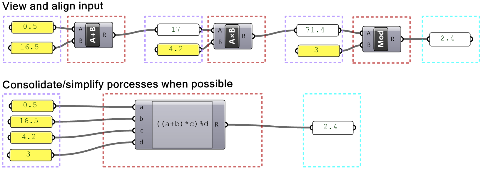
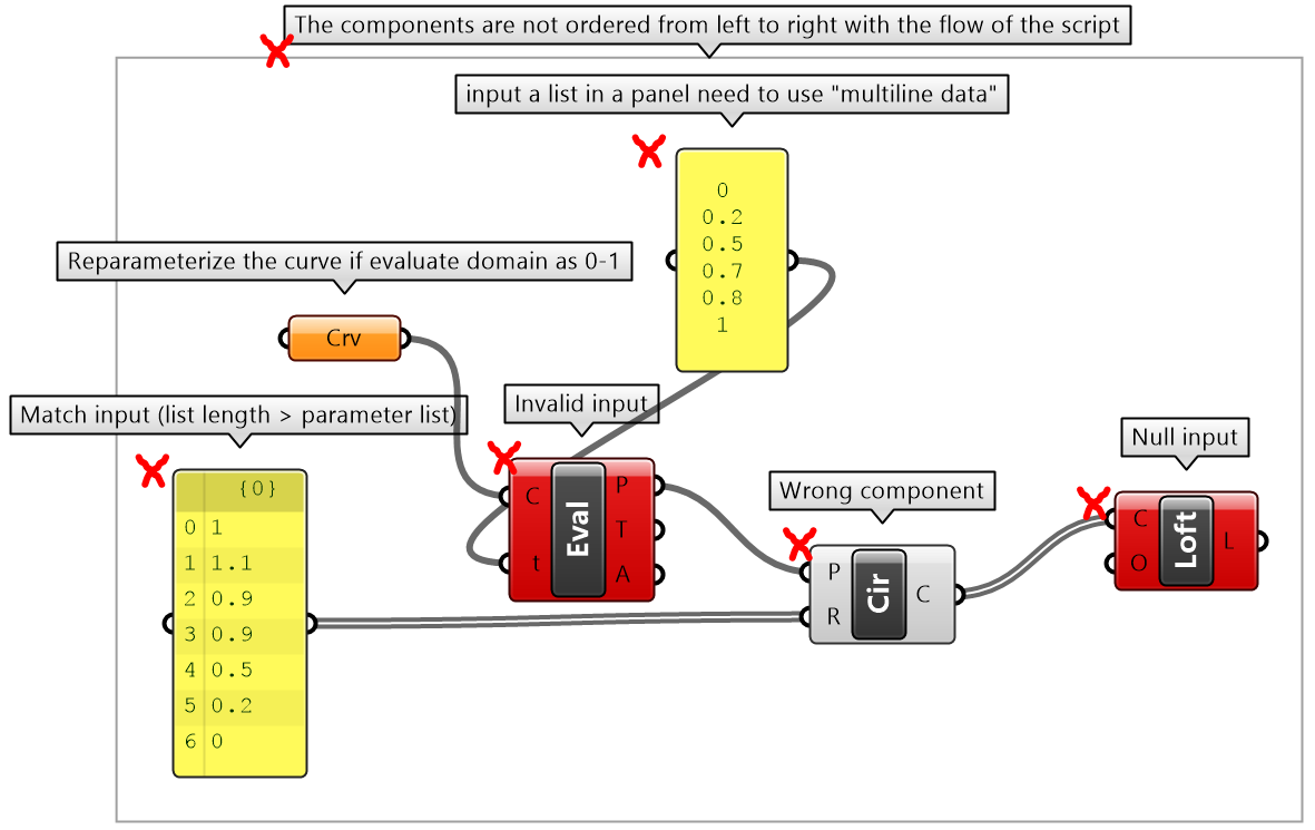
You should try to organize your solutions horizontally or vertically to clearly see the sequence of operations. You should also check the output from each step to make sure it is as expected before continuing on your code. There are also some techniques that help consolidate the script, for example, use Expression when multiple numeric and math operations are involved. The following highlights some unfavorable organization.
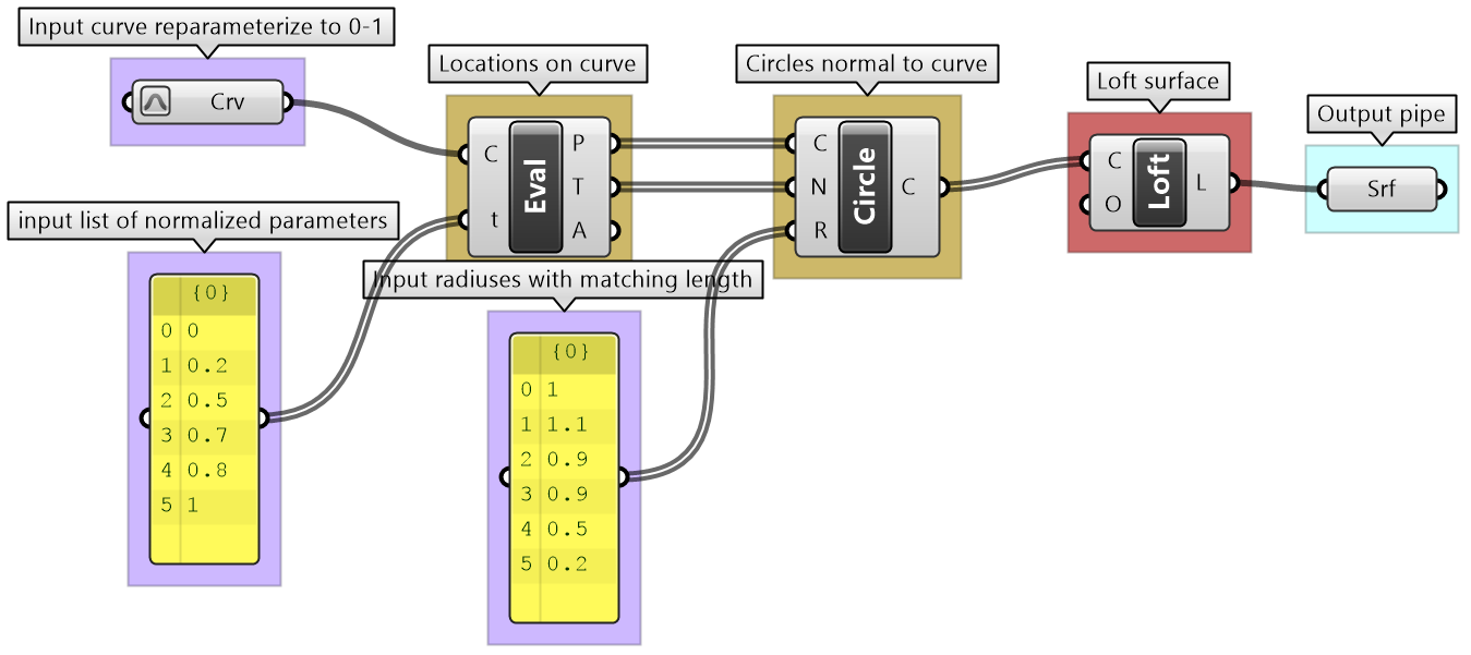
The following shows how to rewrite the same code to make it less error-prone.
Mismatched data structures
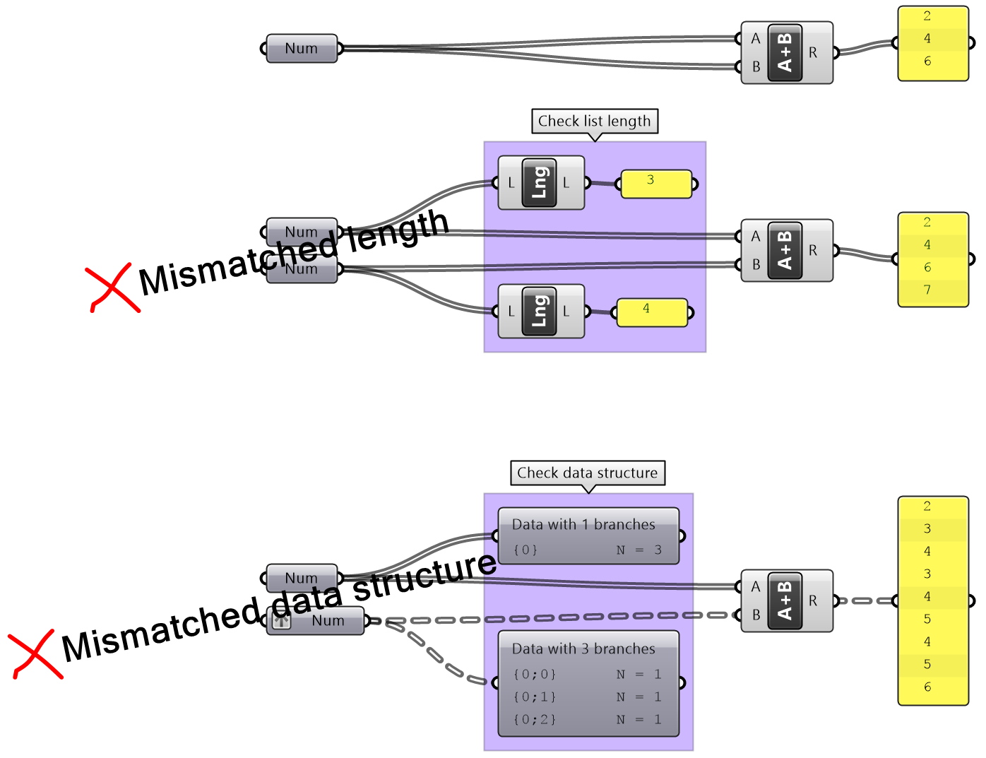
Mismatched data structures as input to the same process or component are particularly tricky to guard against in GH, and has the potential to spiral the solution out of memory. It is essential to test the data structure of all input (except trivial ones) before feeding into any component. It is also important to examine the desired matching under different scenarios (data matching will be explained at length later).
Long processing time
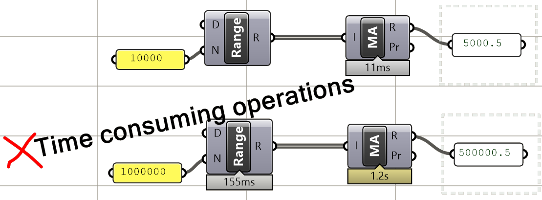
Some algorithms are time-consuming, and you simply have to wait for it to process, but there are ways to minimize the wait when it is unnecessary. For example, at the early cycles of development, you should try to use a smaller set of data to test your solution with before committing the time to process the full set of data. It is also a good practice to break the solution into stages when possible, so you can isolate and disable the time-consuming parts. Also, it is often possible to rewrite your solution to be more optimized and consume less time. Use the GH Profiler to test processing time. When a solution takes far too long to process or crashes, you should do the following: before you reopen the solution, disable it, and disconnect the input that caused the crash.
Poor organization
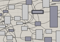
Poorly organized definitions are not easy to debug, understand, reuse or modify. We can’t stress enough the importance of writing your definitions with styles, even if it costs extra time to start with. You should always color code, label everything, give meaningful names to variables, break repeated operations into modules and preview your input and output.
Algorithms tutorials
Unioned circles tutorial
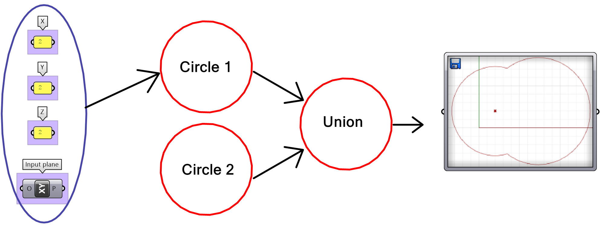
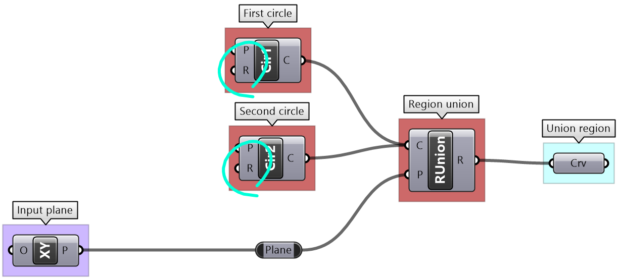
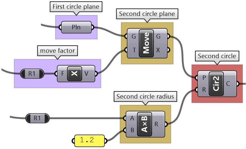
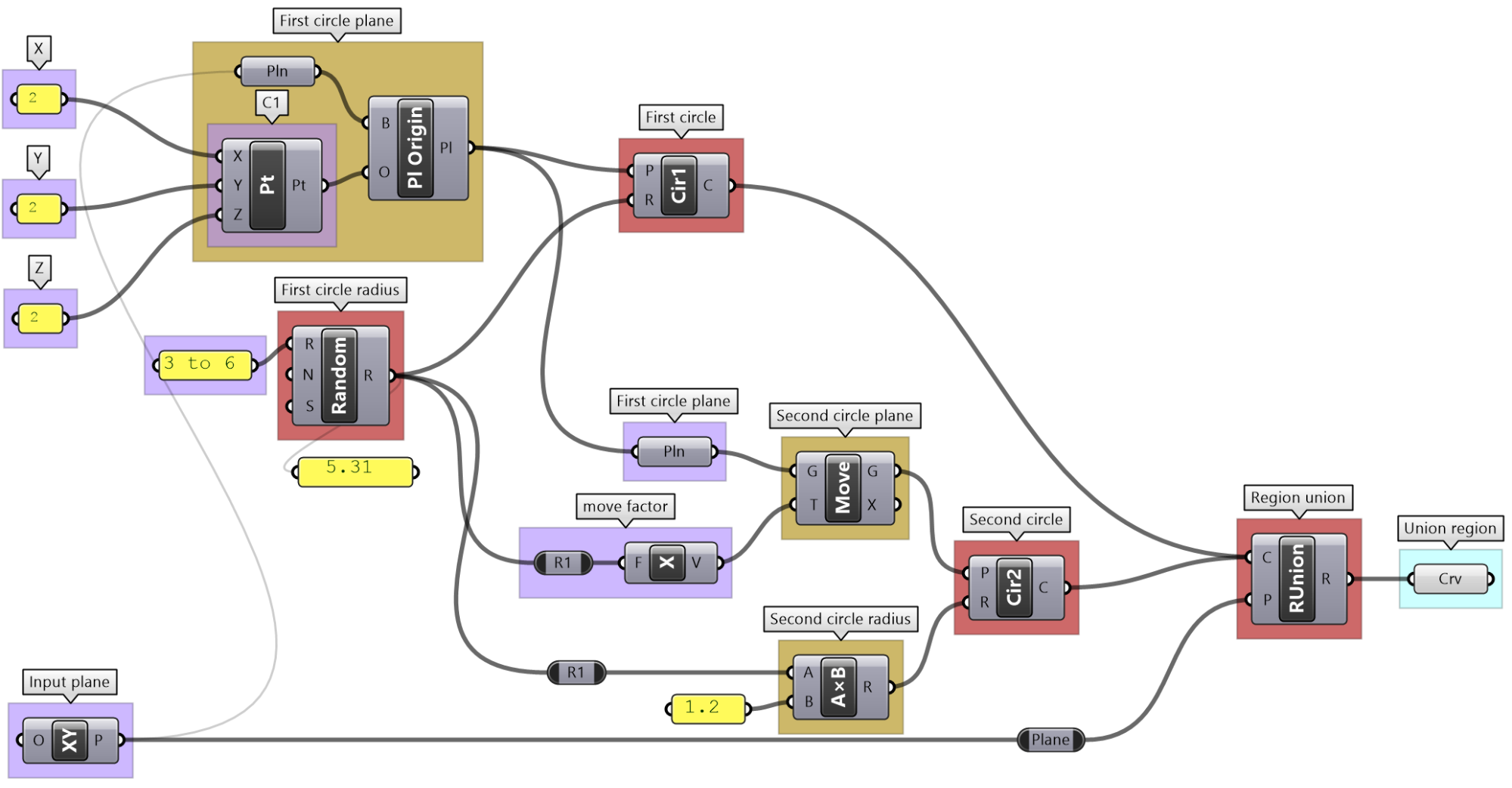
Use the 4-step process to design an algorithm that unions 2 circles, given the following: both are located on the XY-Plane. The first circle (Cir1) has a center (C1) = (2,2,2) and radius (R1) = some random number between 3 and 6. The second circle (Cir2) has a center (C2) is shifted to the right of (Cir1) by an amount equal to R1 along positive X-Axis. R2 = R1 * 1.2
| Analyze the question and the flow of the solution | |
| Output:
Curve for the region union. |
|
| Key Proces: union of 2 circles:
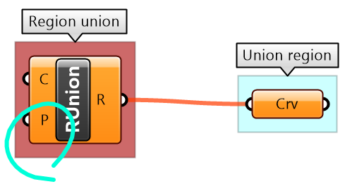
Use the Region Union component that takes curves and a plane. |
|
| Input to the region union:
Identify the input needed and use given input when relevant. The plane for region union has been given. The 2 circles need their own plane and radius. The center of the plane is the center of the circle. |
|
| Intermediate process to generate the center and plane of the 1st circle:
Construct a center from the given coordinates. Create a plane using Plane Origin component and use the constructed center and XY-Plane The radius is from a random number between 3 and 6. Use Random component to create the radius |
|
| Intermediate process to generate the center and plane of the 2nd circle:
Calculate the 2nd circle plane by moving the first circle plane along the xaxis by an amount = first radius GCalculate the 2nd circle radius by multiplying the first radius by 1.2 |
|
Sphere with bounds tutorial
Use the 4-step process to draw a sphere with a radius between 2 and 6. If the input is less than 2, then set the radius to 2, and if the input radius is greater than 6, set the radius to 6. Use a number slider to input the radius and set between 0 and 10 to test. Make sure your solution is well organized, color-coded and labeled properly.
| Use the 4-step process to solve the algorithms | |
| Output:
The sphere as geometry. |
|
| Key Process: create a sphere:
Map the coordinates list from its current domain to a new domain 3 to 9. Use ReMap component |
|
| Input:
1- The radius parameter (0 - 10) 2- The bounds of the radius are 2 & 6 |
|
| Intermediate processes #1:
Construct a selection logic of radii and pattern. The radii is a list of the values from the slider, min and max. The list of pattern is generated to select the correct radius value. |
|
| Intermediate processes #2
The selection logic checks if the radius from the slider is between the bounds, then set it to be selected, if less, then select the min, and if more select the max. |
|
Data operations tutorial
Given the numbers embedded in the Number parameter below:
1- Analyze input in terms of bounds and distribution
2- View the data and how it is structured
3- Extract even numbers
4- Sort numbers descending
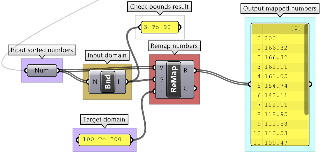
5- Remap sorted numbers to (100 to 200)
| Solution | |
| 1 - Analyze the input bounds and distribution
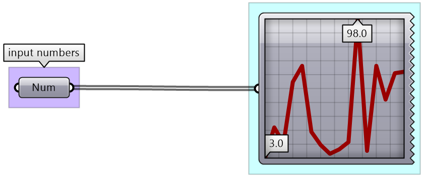
Use the QuickGraph to show that the set of numbers are between 3 and 98 and are distributed randomly. |
|
| 2 - Analyze the input data structure and values
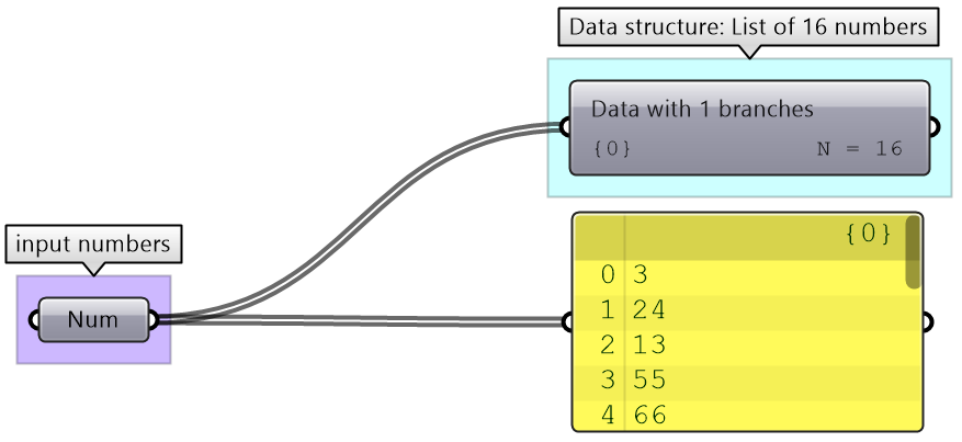
Use the Panel and Parameter Viewer to show there are 16 elements organized in a list |
|
| 3 - Extract Even numbers:
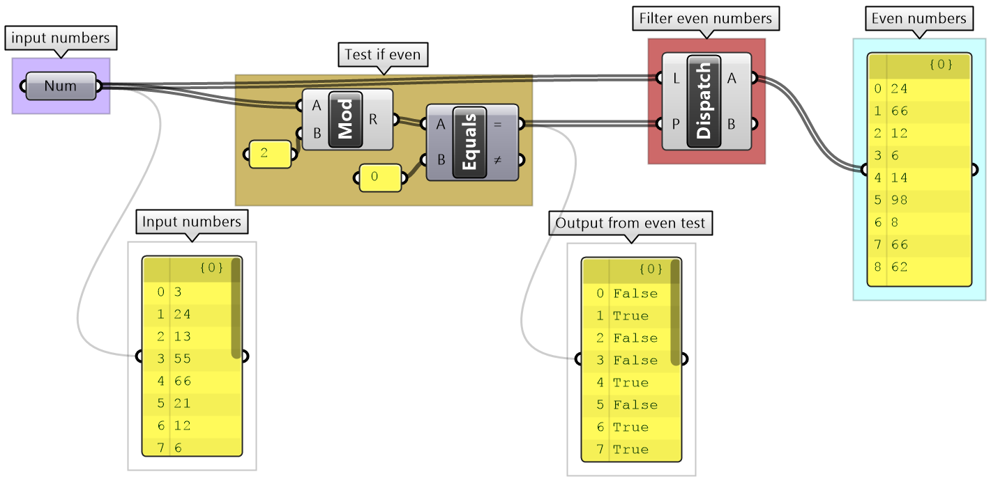
Create the logic to test if a number is even (divisible by 2 without a remainder) and use Dispatch to extract even numbers |
|
| 4 - Sort numbers descending
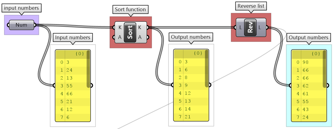
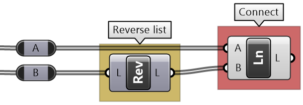
The Sort List component sorts numbers in ascending order. Use Reverse List component to further process the list to order descending |
|
| 5 - Remap to 100-200
Check the input range and use Remap component to scale data to be between 100-200 |
|
Pitfalls tutorial
Analyze what the following algorithm is intended to do, identify the errors that are preventing it from working as intended, then rewrite to fix the errors. Organize to reflect the algorithm flow, label, and color-code.
| Solution | |
| Mark the errors: | |
| Fix the errors and rewrite the solution with labels: | |
Chapter Two: Introduction to Data Structures
All algorithms involve processing input data to generate a new set of data as output. Data is stored in well-defined structures to help access and manipulate efficiently. Understanding these structures is the key to successful algorithmic designs. This chapter includes an in-depth review of the basic data structures in Grasshopper.
Overview
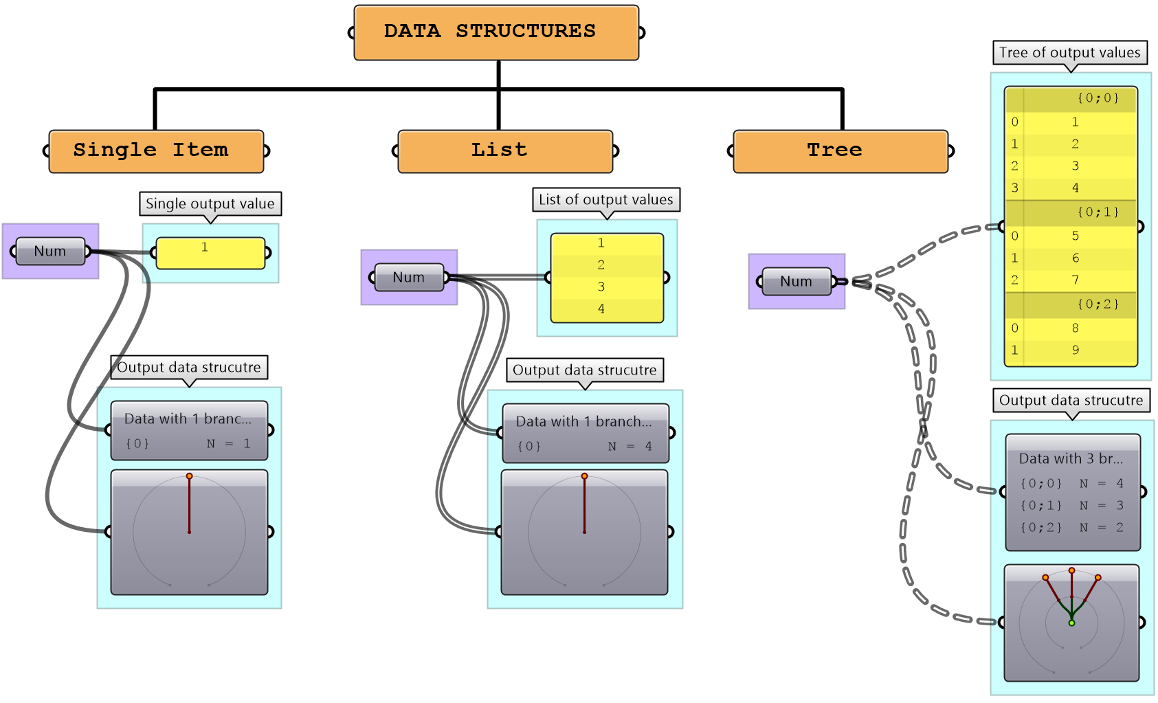
Grasshopper has three distinct data structures: single item, list of items and tree of items. GH components execute differently based on input data structures, and hence it is essential to be fully aware of the data structure before using. There are tools in GH to help identify the data structure.
Those are Panel and Param Viewer.
Processes in GH execute differently based on the data structure. For example, the Mass Addition component adds all the numbers in a list and produces a single number, but when operating on a tree, it produces a list of numbers representing the sum of each branch.
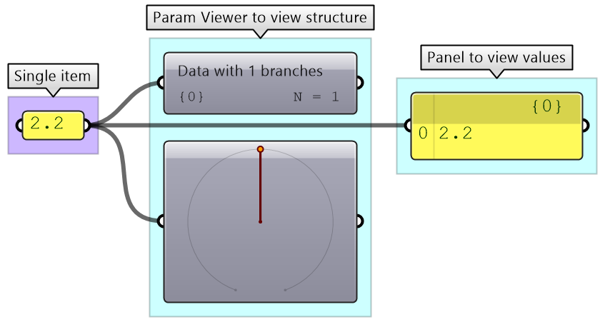
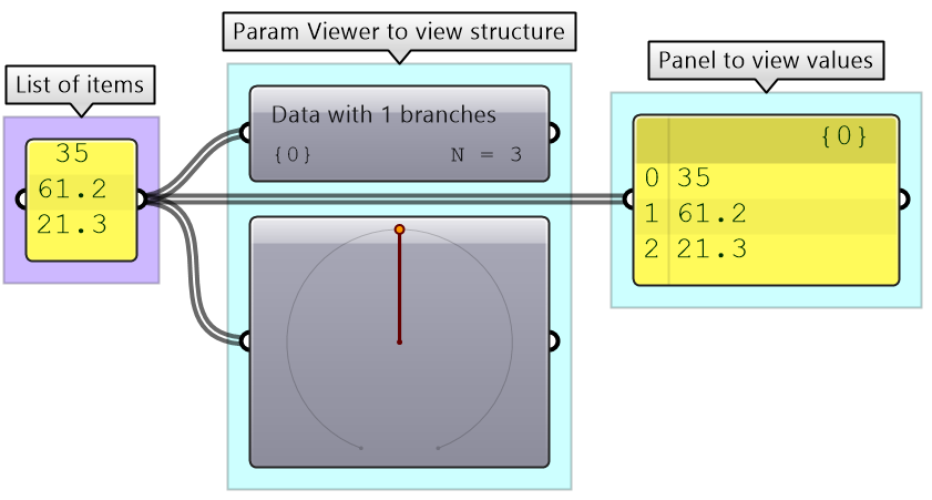
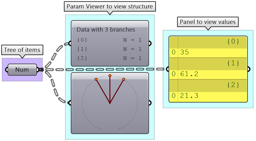
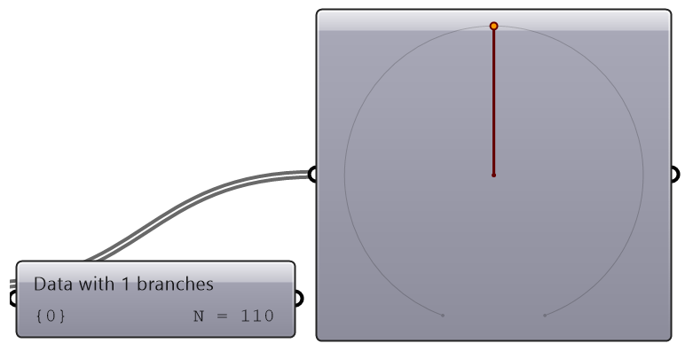
The wires connecting the data with components in GH offer additional visual reference to the data structure. The wire from a single item is a simple line, while the wire connecting a list is drawn as a double line. A wire output from a tree data structure is a dashed double line. This is very useful to quickly identify the structure of your data.
| Display the data structure | Example |
|
Item: single branch with single item Wire display: single line Map the coordinates list from its current domain to a new domain 3 to 9. Use ReMap component |
|
|
List: single branch with multiple items Wire display: double line |
|
|
Tree: multiple branches with any number of items per branch Wire display: double dashed line |
Generating lists
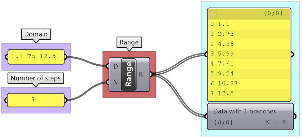
There are many ways to generate lists of data in GH. So far we have seen how to directly embed a list of values inside a parameter or a panel (with multiline data). There are also special components to generate lists. For example, to generate a list of numbers, there are three key components: Range, Series, and Random. The Range component creates an equally spaced range of numbers between a min and max values (called domain) and a number of steps (the number of values in the resulting list is equal to the number of steps plus one).
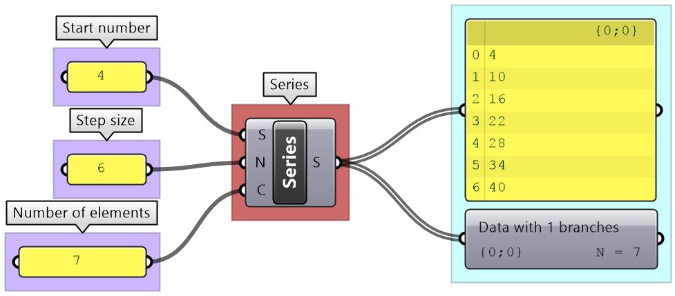
The Series component also creates an equally spaced list of numbers, but here you set the starting number, step size and the number of elements.
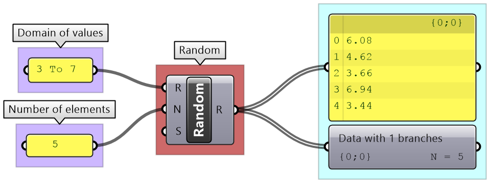
The Random component is used to create random numbers using a domain and a number of elements. If you use the same seed, then you always get the same set of random numbers.
Lists can be the output of some components such as Divide curve (the output includes lists of points, tangents and parameters). Use the Panel component to preview the values in a list and Parameter Viewer to examine the data structures.
Generating lists tutorial
| Description | Grasshoper Solution |
|
Directly set a circle in a parameter. |
|
|
Set the plane input to the default XY-Plane (internal). Supply a list of radiuses using Range component. |
|
|
Supply one value for the center. Normal is set to default (internal). List of radiuses using Random component. |
|
|
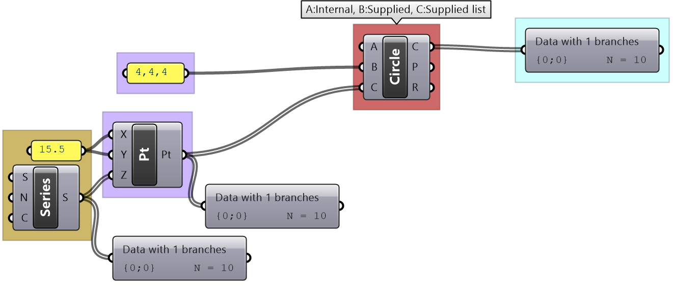
Circle from 3 points: A: set internally to one value B: Supply one value C: Supply a list of values using the Series component to set a list of Z coordinates |
List operations
GH offers an extensive list of components for list operations and list management. We will review a few of the most commonly used ones.
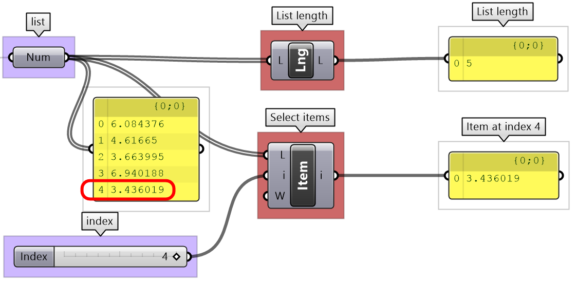
You can check the length of a list using the List Length component, and access items at specific indices using the List Item component.
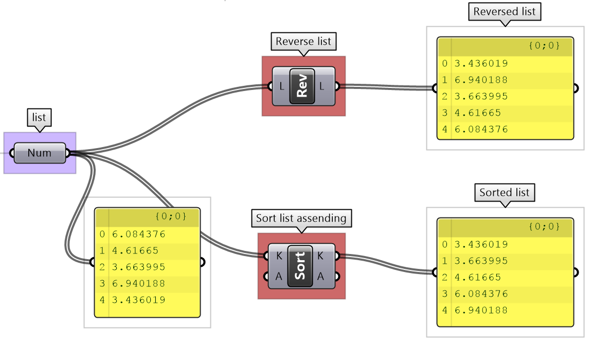
Lists can be reversed using the Reverse List component and sorted using the Sort List component.
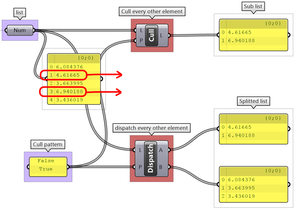
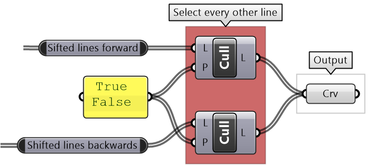
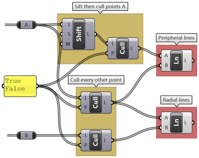
Components such as Cull Patterns and Dispatch allow selecting a subset of the list, or splitting the list based on a pattern. These components are very commonly used to control data flow and select a subset of the data.
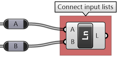
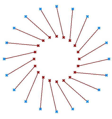
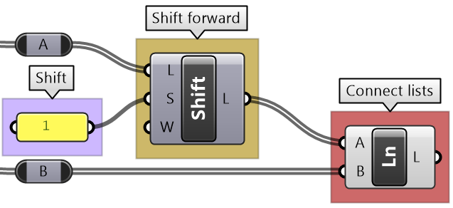
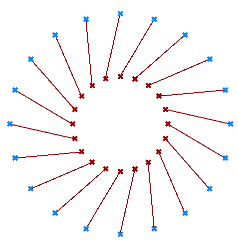
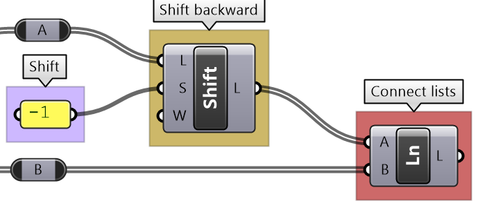
The Shift List component allows shifting a list by any number of steps. That helps align multiple lists to match in a particular order.
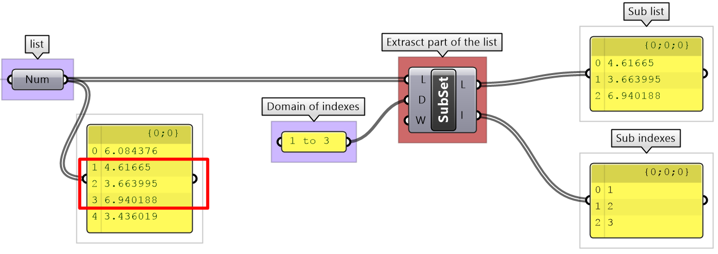
The Subset component is another example to select part of a list based on a range of indices.
List operations tutorial
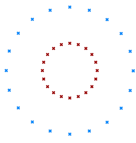
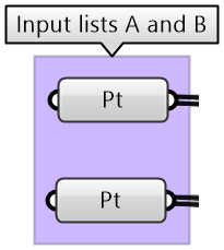
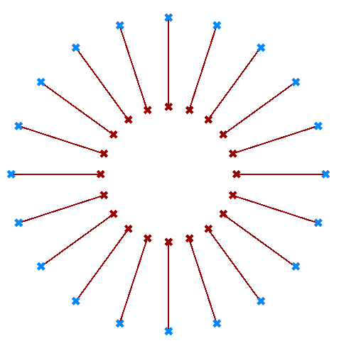
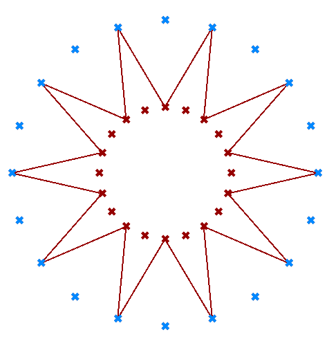
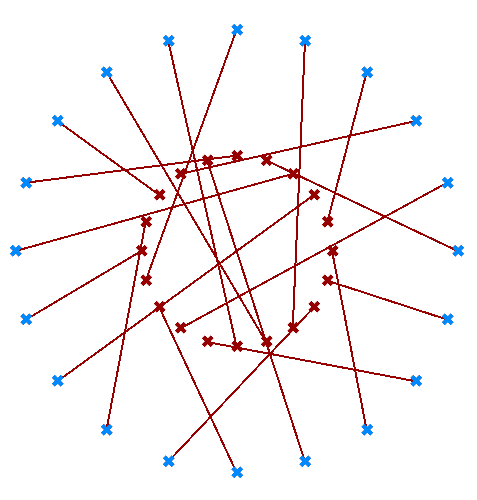
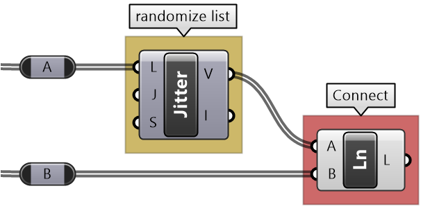
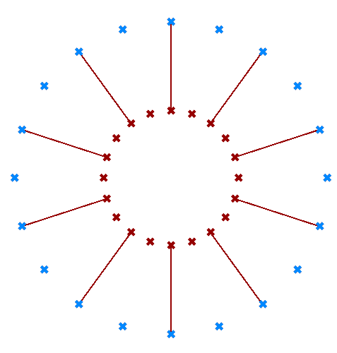
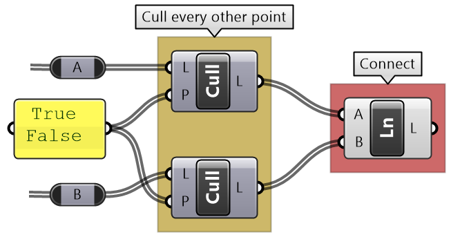
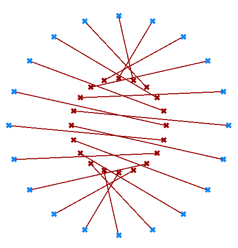
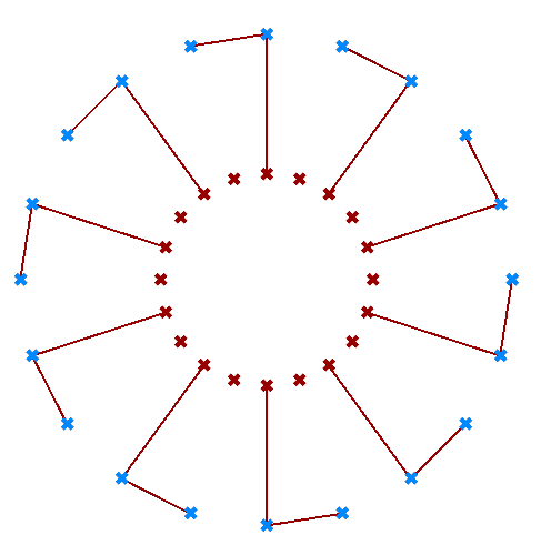
Use the two given lists of points to generate the following images.
| Output Image | Grasshoper Solution |
List matching
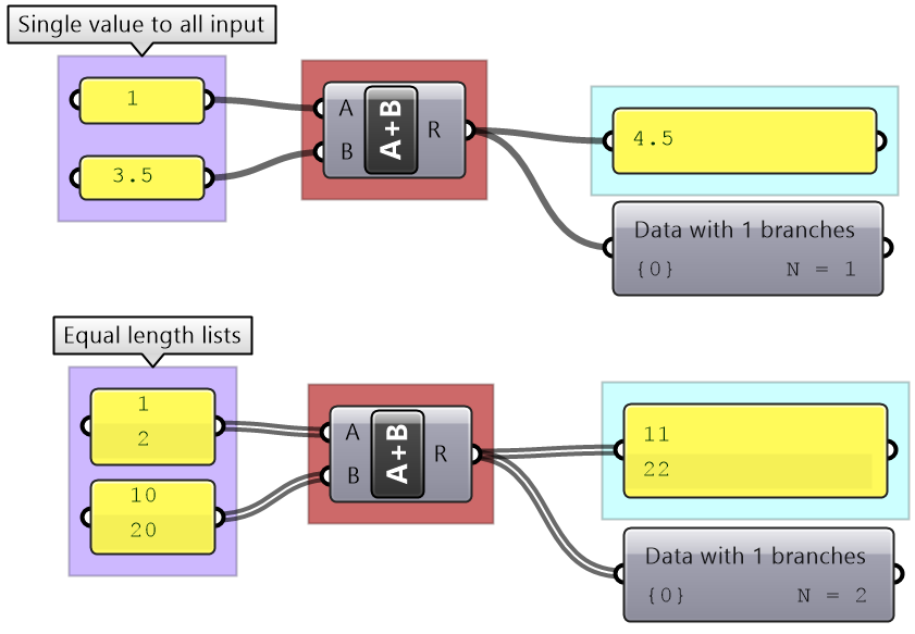
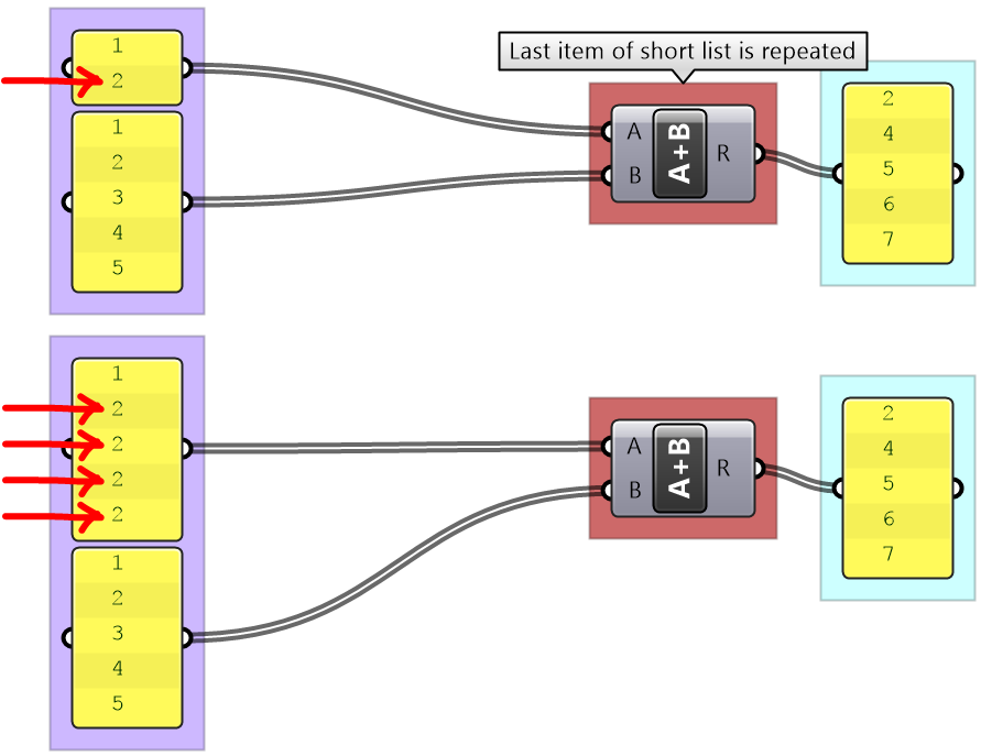
When the input is a single item or has an equal number of elements in a simple list, it is easy to imagine how the data is matched. The matching is based on corresponding indices. Let’s use the Addition component to examine list matching in GH.
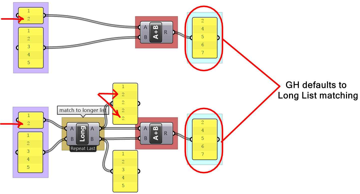
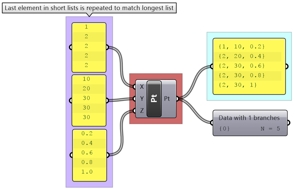
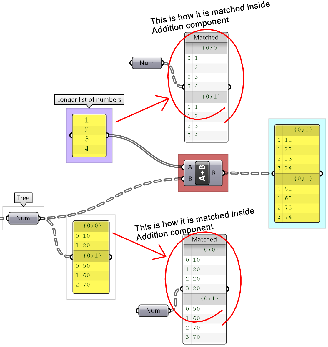
There are times when the input has variable length lists. In this case, GH reuses the last item on the shorter list and matches it with the next items in the longer list.
Grasshopper offers alternative ways of data matching: Long, Short, and Cross reference that the user can force to use. The Long matching is the same as the default matching. That is the last element of the shorter list is repeated to create a matching length.
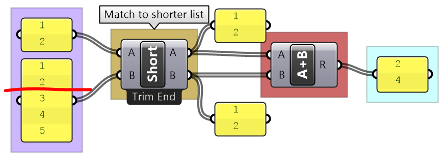
The Short list matching truncates the long list to match the length of the short list. All additional elements are ignored and the resulting list has a length that matches the shorter list.
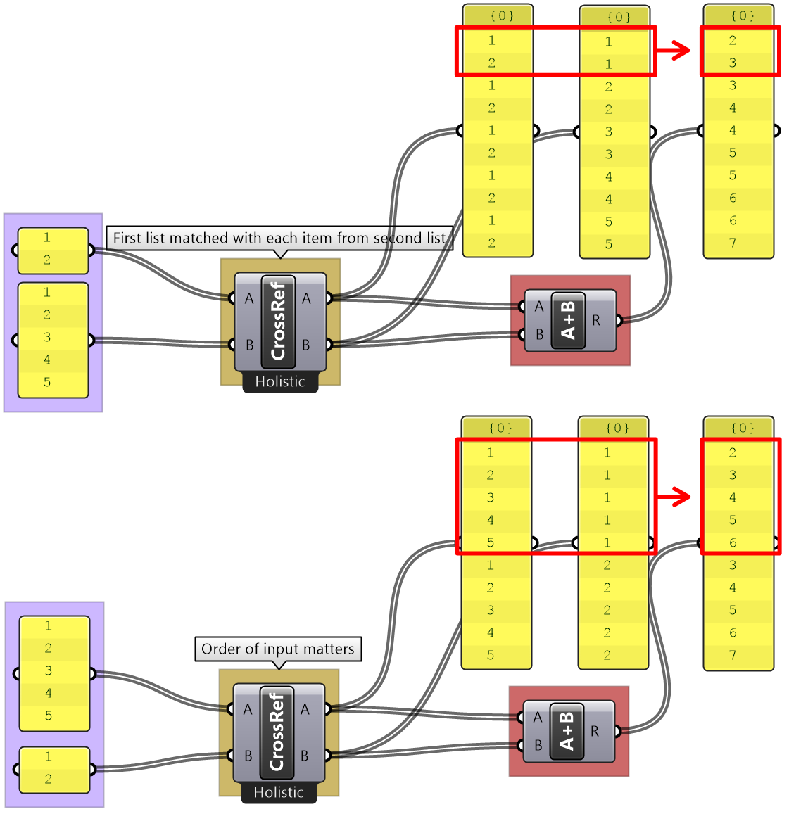
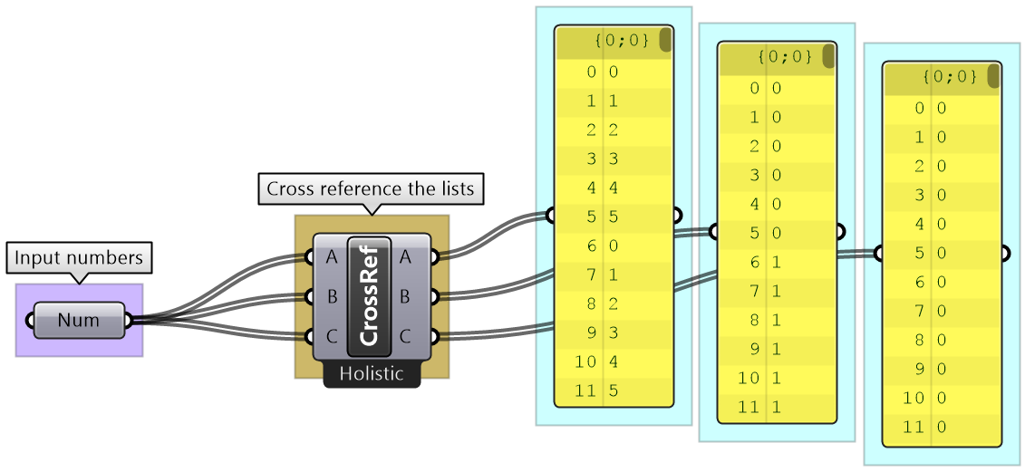
The Cross Reference matches the first list with each of the elements in the second list. The resulting list has a length equal to the multiplication product of the length of input lists. Cross reference is useful when trying to produce all possible combinations of input data. The order of input affects the order of the result as shown in Figure (49).
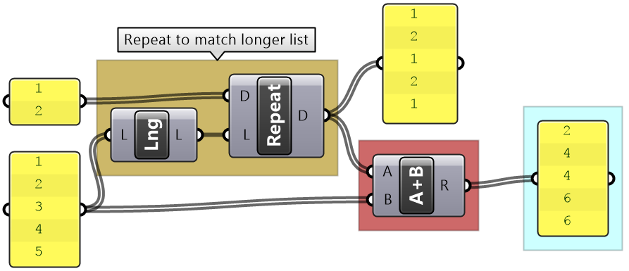
If none of the matching methods produce the desired result, you can explicitly adjust the lists to match in length based on your requirements. For example, if you like to repeat the shorter list until it matches the length of the longer list, then you’ll need to create the logic to achieve that as in the following example.
List matching tutorial
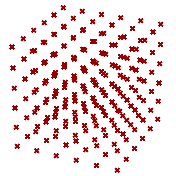
Use the input list of 6 numbers to construct the points in the image.
| Solution | |
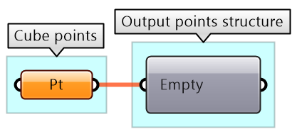
| Output:A list of 6x6x6 = 216 points constructed from a list of X, Y, Z coordinates. | |
| Key process: Use the Construct Point component to generate the list of points. | |
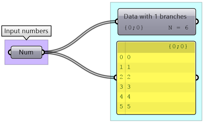
| Input: Examine input using the Parameter Viewer and Panel components. The given list has 6 points representing each coordinate along each axis. | |
| Intermediate process: Need to find all possible permutations for the coordinates to create the cube of 216 points along all 3 axes.
Use Cross Reference matching to generate lists of coordinates that have all possible permutations. | |
| Put it all together | |
Data structures tutorials
Variable thickness pipe tutorial
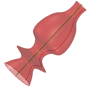
Create a surface similar to the one in the image with a thickness that changes in 10 locations random along the curve. Thickness variations are random between 1 and 3.
| Algorithm analysis | |
|
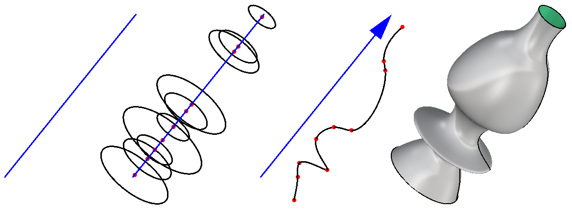
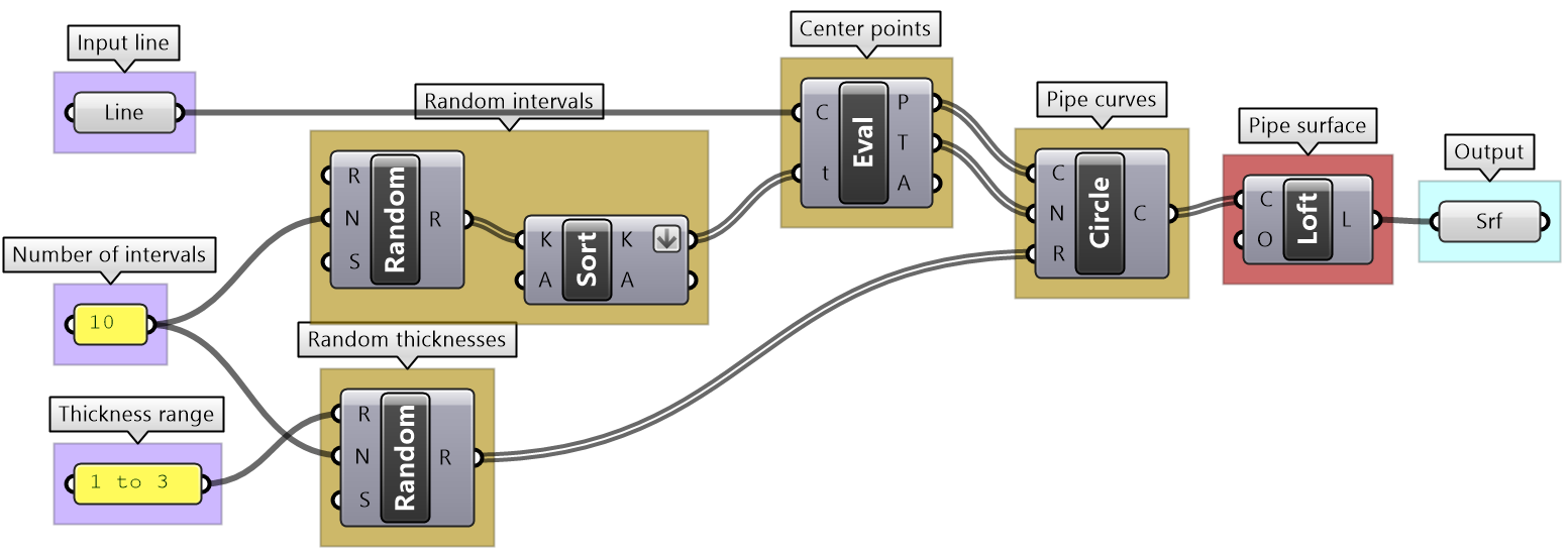
To figure out an algorithm, it is useful to think in terms of 3D modeling. There are 2 ways to generate this surface: 1- Create circles along the line at random locations with random radius, then loft the result. 2- Figure out the profile curve and revolve along the line The first process goes like this: 1- Divide the line at random locations 2- Orient to the planes at locations (line normal to planes) 3- Create the circles (or points for the profile curve) 4- Select the circles (in order) to Loft (or Interpolate Curve then Revolve) |
|
| Solution steps | |
|
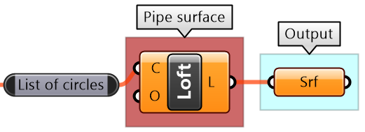
Output: The surface |
|
|
Key process: Use the Loft component to generate the surface |
|
|
Input: Line, Number of intervals and Thickness range |
|
|
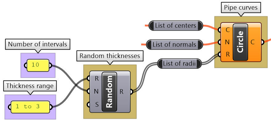
Intermediate process #1: The Loft is created from a list of circles. Use the Circle component that takes centers, normals and radii lists. We can use the default Loft options. |
|
|
Intermediate process #2: List of radii is created randomly. Use the Random component and the input thickness range. |
|
|
Intermediate process #3: Evaluate the line at random intervals. Use the Evaluate Curve component to extract points and normals, and use the Random component to generate the parameters along the curve. Problem: the random parameters are not ordered and hence produce unordered points. Use the Sort List component to order the parameters before feeding into the Evaluate Curve. |
|
| Put it all together | |
Custom matching tutorial
Explain the default GH list matching in the following example. Compare the result with "Shortest List" matching, then try to create a custom matching that repeats the pattern of the shorter lists. E.g. [1,2] becomes [1,2,1,2,...] until it matches the length of the longer list.
| Solution | |
|---|---|
|
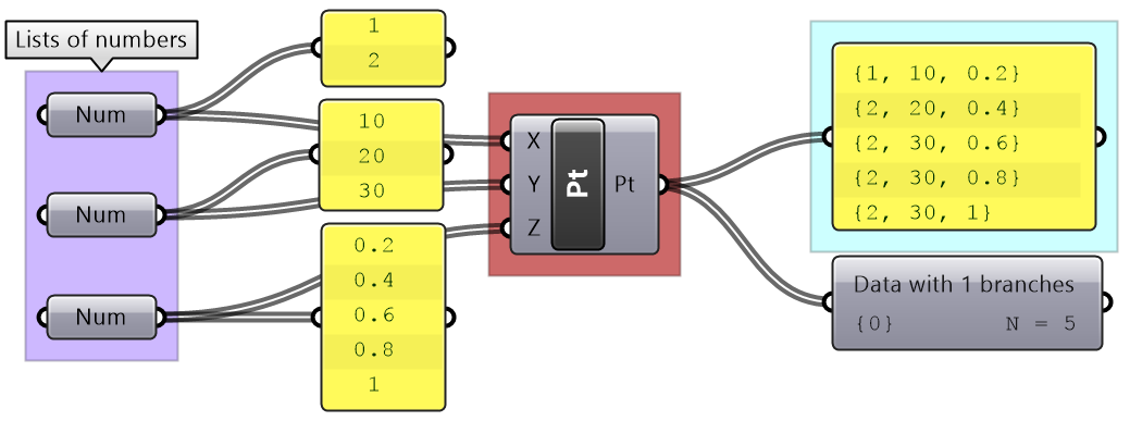
Construct default GH matching: To test the matching, fill the lists as coordinates to a Construct Point component and observe the result. |
|
|
Analysis of GH default matching: The last element of shorter lists is repeated until all lists have the same length, then elements are matched by indices. |
|
|
Shortest List matching: Omit additional values in longer lists so that the length of all lists equals the length of the shortest list. |
|
|
Custom matching: Use the Repeat component to repeat the elements until match the length of the longest list. |
|
Simple truss tutorial
Create a simple truss as in the image. Use given baseline, height, number of runs and joint radius.
| Algorithm analysis | |
|---|---|
|
Identify the desired output for the truss: |
|
|
Define the input: L= line geometry on xy-plane H= height R= number of runs J= joint radius |
|
|
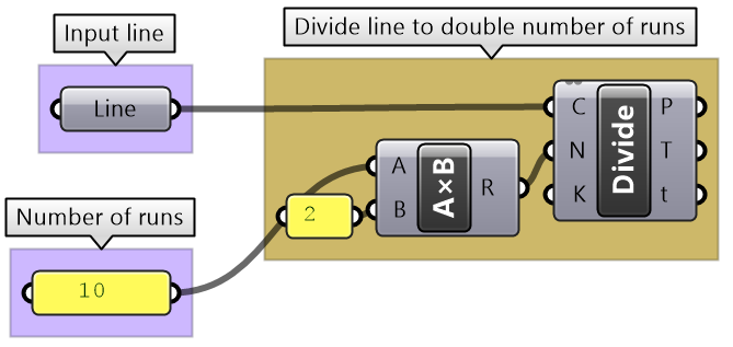
Divide curve by 2*R: |
|
|
Move every other point in the Z direction by height. |
|
|
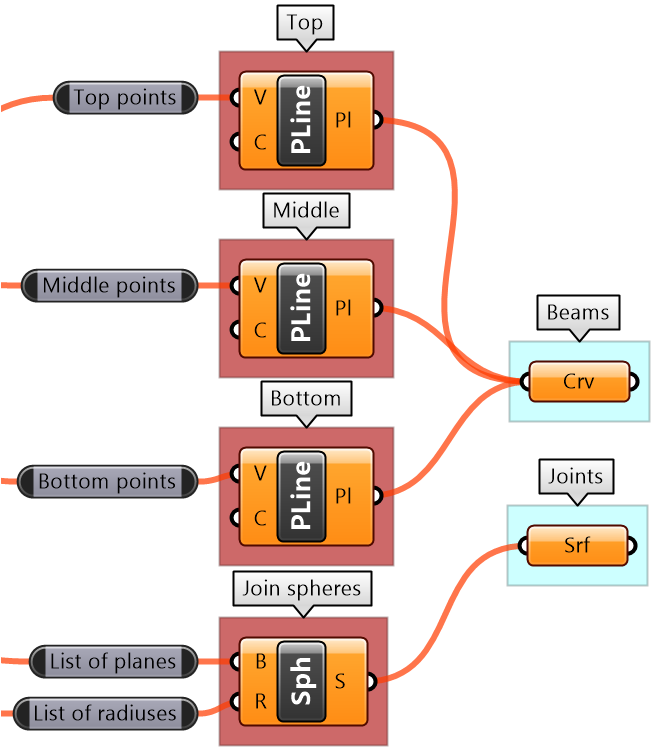
Create 3 sets of ordered points for the bottom beams, top beams and middle beams, then connect each of the 3 sets with a polyline. |
|
| Algorithm implementation in Grasshopper | |
|---|---|
|
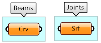
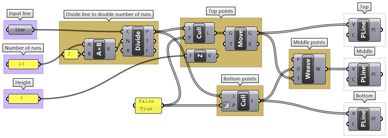
Output: There are 2 outputs, the beams as curves (polylines) and joints as spheres (surfaces) |
|
|
Key processes: Need to create the polylines for the top, middle, and bottom beams. Use the Polyline component with relevant set of points for each. Use the Sphere component to create joints. Use middle points and joint radius as input. |
|
|
Given input: Four given input: line, number of runs, height and joint radius. |
|
|
Intermediate process #1: Divide the curve with twice the number of runs. Use Divide Curve component and Multiply the number of runs. |
|
|
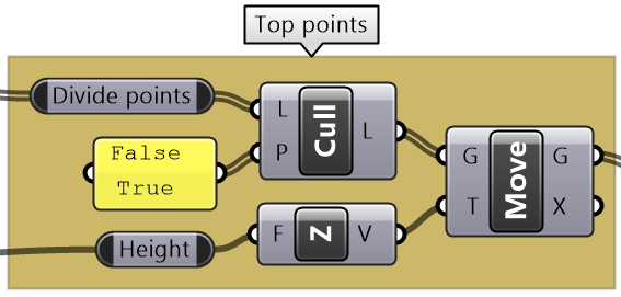
Intermediate process #2: To create top points, select every other point from the list of all divide points, then move vertically by the height amount. Use Cull Pattern component to select points and Move component to shift vertically. |
|
|
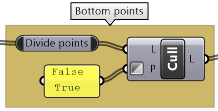
Intermediate process #3: To create bottom points, select every other point, in the invert pattern used to select top points. Use Cull Pattern component to select points (set invert flag for the pattern input). |
|
|
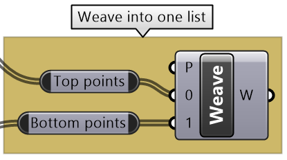
Intermediate process #4: To create middle points, Weave the top and bottom points. |
|
| Put it all together. | |
|---|---|
Pearl necklace tutorial
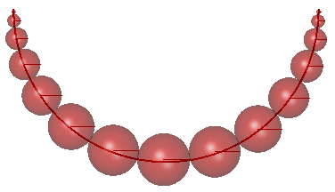
Create a necklace with one big pearl in the middle, and gradually smaller size pearls towards the ends as in the image. Make the number of pearls parametric between 15-25.
| Algorithm analysis | |
|---|---|
|
The workflow to create the necklace follows these general lines: 1. Divide the curve into segments of variable distances (widest in the middle and narrow towards the ends. 2. Find midpoints for each segment and its length. 3. Create spheres at centers using half the length as radius. |
|
| Solution steps | |
|---|---|
|
Output: The surfaces. |
|
|
Key process: Use the Sphere component to generate the surfaces. |
|
|
Given input: Necklace curve, Number of pearls as a parameter (can be changed by the user) |
|
|
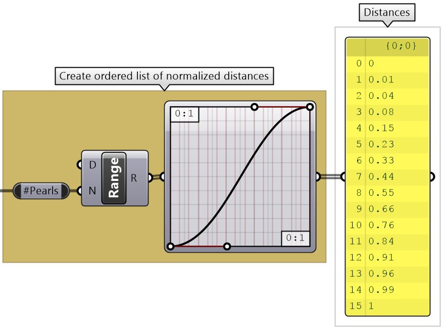
Intermediate process #1: The Range component creates equal distances. We need to change to variable distances and for that we can use the Graph Mapper component to control the spacing. |
|
|
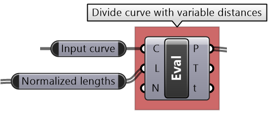
Intermediate process #2: Since we have normalized distances from the start of the curve (parameters are between 0 to 1), we can use the Evaluate Length component to find the divide points. |
|
|
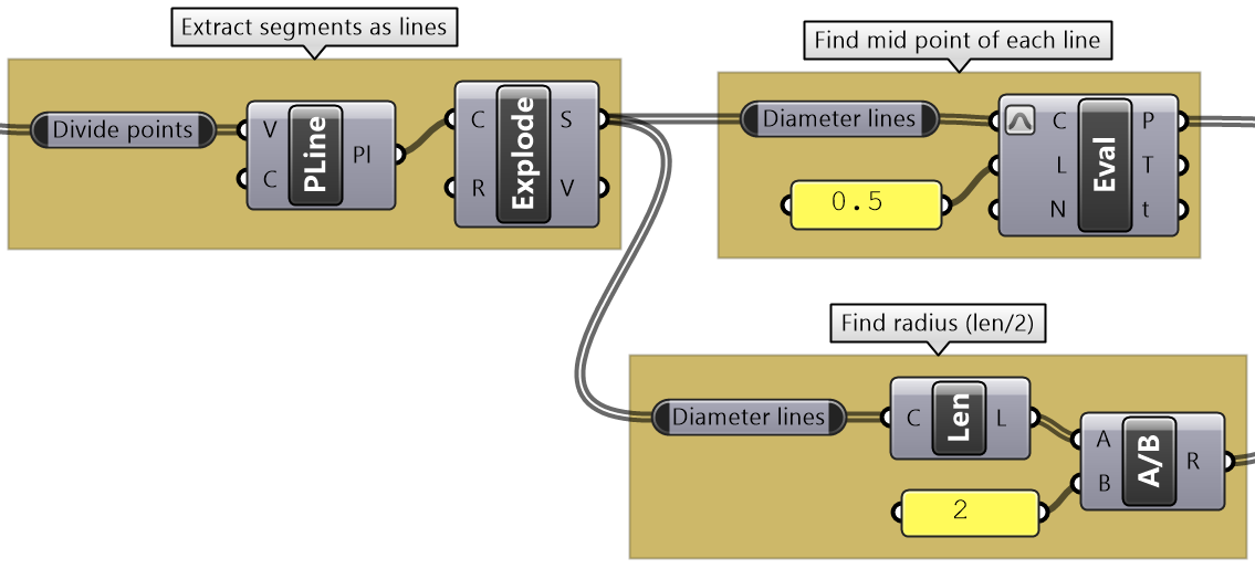
Intermediate process #3: Generate the segments. Use Polyline and Explode components to turn the points into segments. Center points are calculated at the middle of the segments. Use Evaluate Length at mid length. Radii is calculated as half of each segment length. Use Length and Division components. |
|
| Put it all together. | |
|---|---|
Chapter Three: Advanced Data Structures
This chapter is devoted to the advanced data structure in GH, namely the data trees, and different ways to generate and manage them. The aim is to start to appreciate when and how to use tree structures, and best practices to effectively use and manipulate them.
The Grasshopper data structure
Introduction
In programming, there are many data structures to govern how data is stored and accessed. The most common data structures are variables, arrays, and nested arrays. There are other data structures that are optimised for specific purposes such as data sorting or mining. In Grasshopper, there is only one structure to store data, and that is the data tree. Hold on, what about what we have learned so far: single item and list of items? Well, in GH, those are nothing but simple trees. A single item is a tree with one branch, that has one element, and a list is a tree with one branch that has a number of elements. It is actually pretty elegant to be able to fit all data in one unifying data structure, but at the same time, this requires the user to be aware and vigilant about how their data structure changes between operations, and how that can affect intended results. This chapter attempts to demystify the data tree of Grasshopper.
Processing data trees
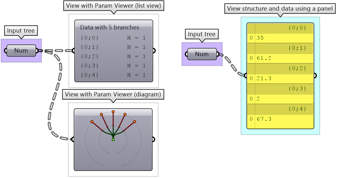
We used the Panel and Parameter Viewer components to view the data structure. We will use both extensively to show how data is stored. Let’s start with a single item input. The Parameter Viewer has two display modes, one with text and one that is graphical. You can see that the single item input is stored in one branch that has only one item.
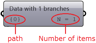
The Parameter Viewer shows each branch address (called “Path”), and the number of elements in that branch as shown in Figure 3.1.2.2.
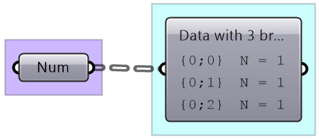
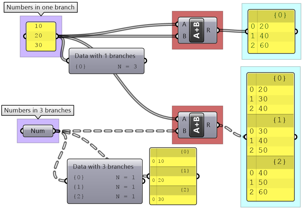
A list of items is typically stored in a tree with one branch. Figure 3.1.2.3. However, the three items can also be stored in three different branches, see Figure 3.1.2.4.
The key to understanding the Grasshopper data structure is to be able to answer the following question: What is the significance of storing the 3 numbers in one branch vs 3 branches? The data structure informs GH components about how to match input values. In other words, components may process data differently based on their structure. The following example illustrates how different data structures for the same set of values can affect the result.
We will elaborate on data tree matching later, but you can already see that GH components do pay attention to the data structure and the result can vary considerably based on it. This is one of the complications inherited in using one unifying data structure in a programming language.
Data tree notation
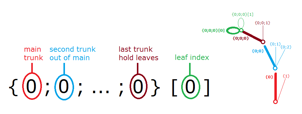
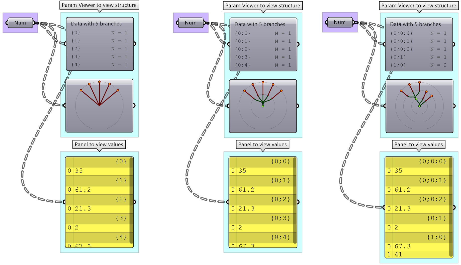
The first step to understanding data trees is to learn the GH notation of trees. As we have seen from the examples, trees consist of branches, and each branch holds a number of elements. The address or path of each branch is represented with integers separated by semicolons and enclosed in curly brackets. The index of each element is enclosed by square brackets. This diagram shows a breakdown of the address of elements in trees.
Here are a few examples of various trees structures and how they show in the Paramster Viewer and the Panel.
Data tree tutorial
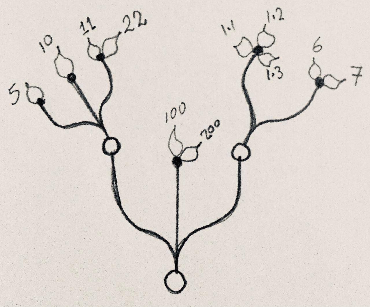
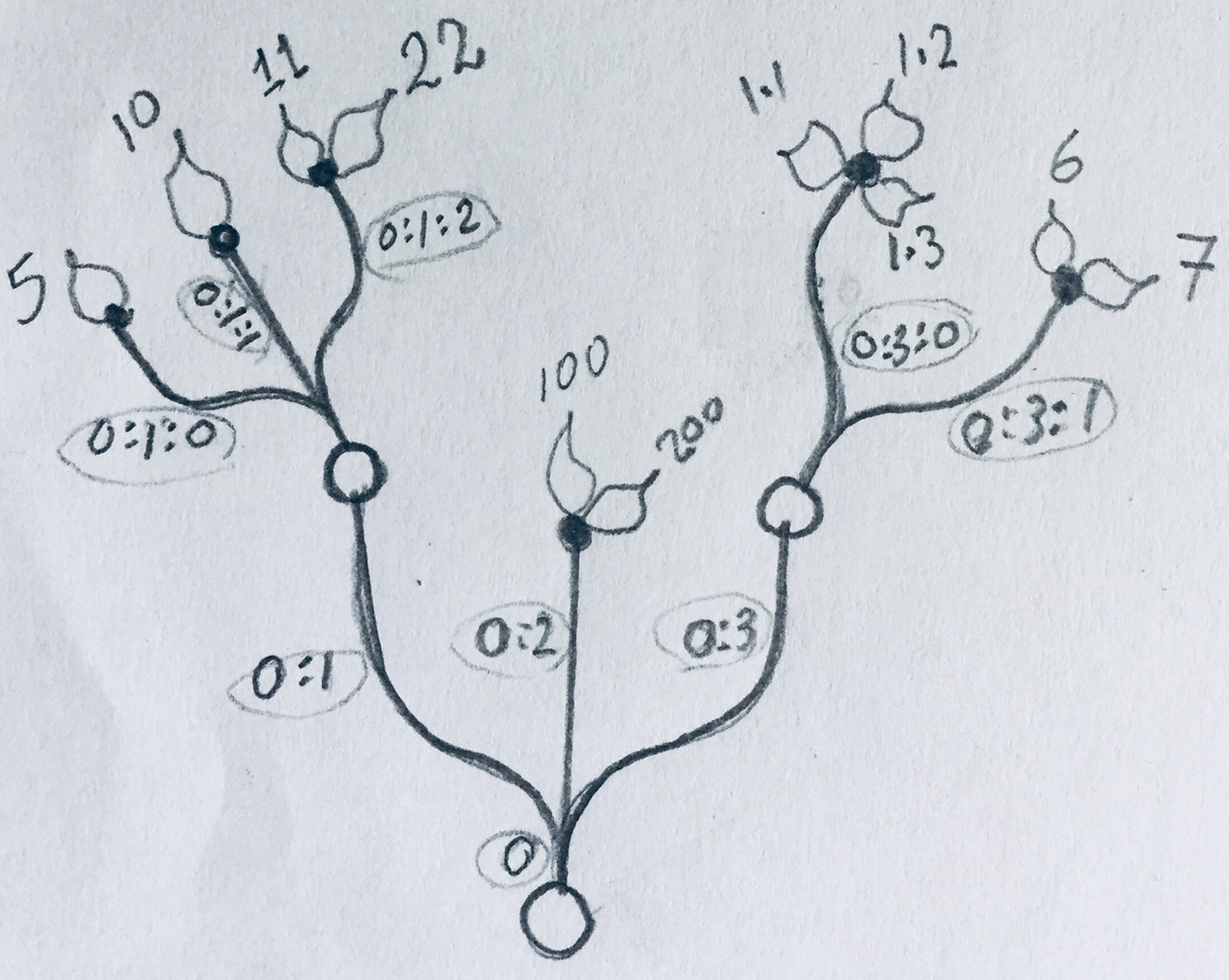
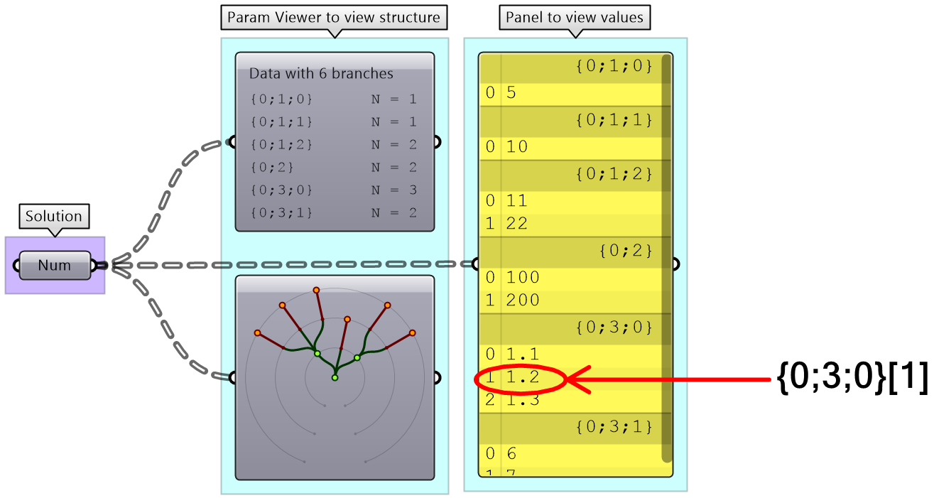
Construct a tree of numbers using the Number parameter, that look similar to the image when viewed in the Param Viewer and contains the numbers indicated. Then type in a Panel the full address to the item "1.2" . Note that order of branches and leaves is always from left to right going clockwise
|
Solution | |
|---|---|
|
The path for “1.2” is: { 0 ; 3 ; 0} [ 1 ] Note: The three branches from the main trunk are set here to 0:1, 0:2, and 0:3. They also could have been 0:0, 0:1 and 0:2. Both are correct. | |
Generating trees
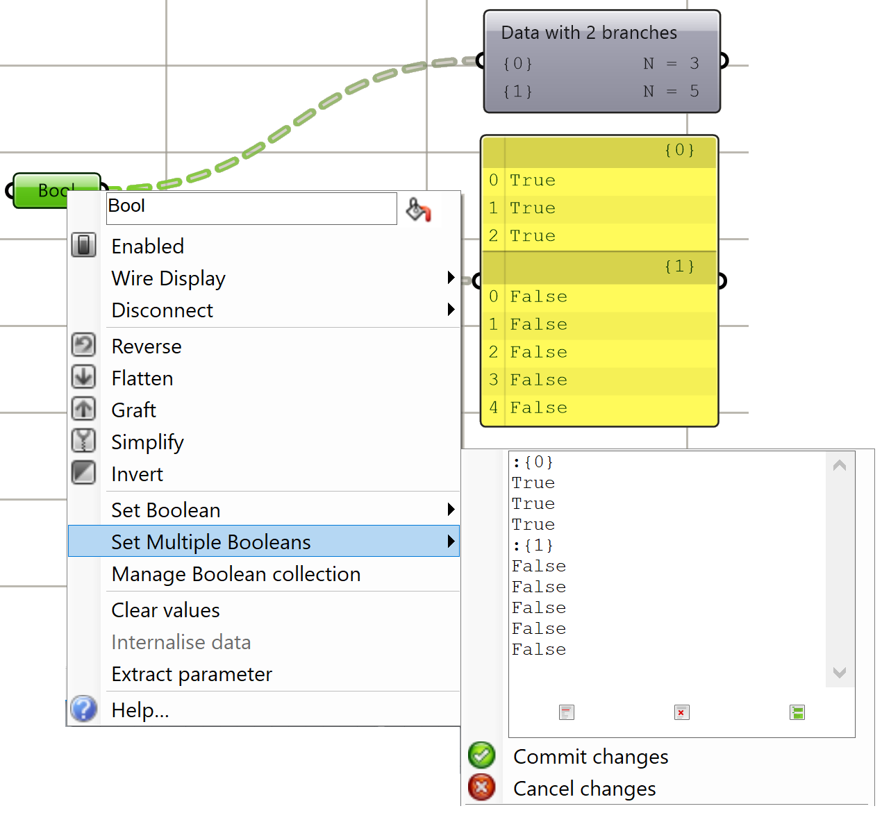
There are many ways to generate complex data trees. Some explicit, but mostly as a result of some processes, and this is why you need to always be aware of the data structures of output before using it as input downstream. It is possible to enter the data and set the data structure directly inside any Grasshopper parameter. Once set, it is relatively hard to change and therefore is best suited for a constant input. The following is an example of how to set data tree directly inside a parameter.
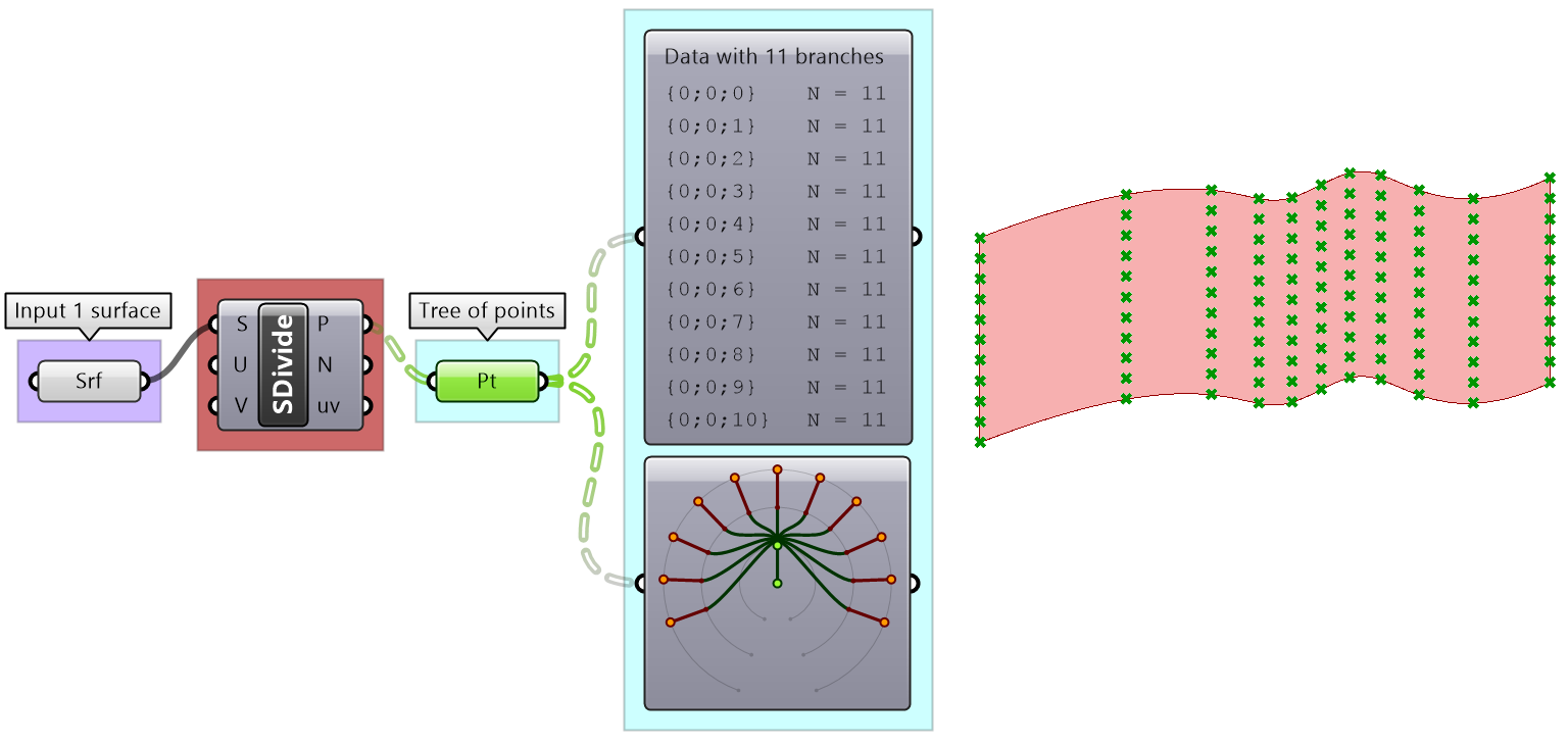
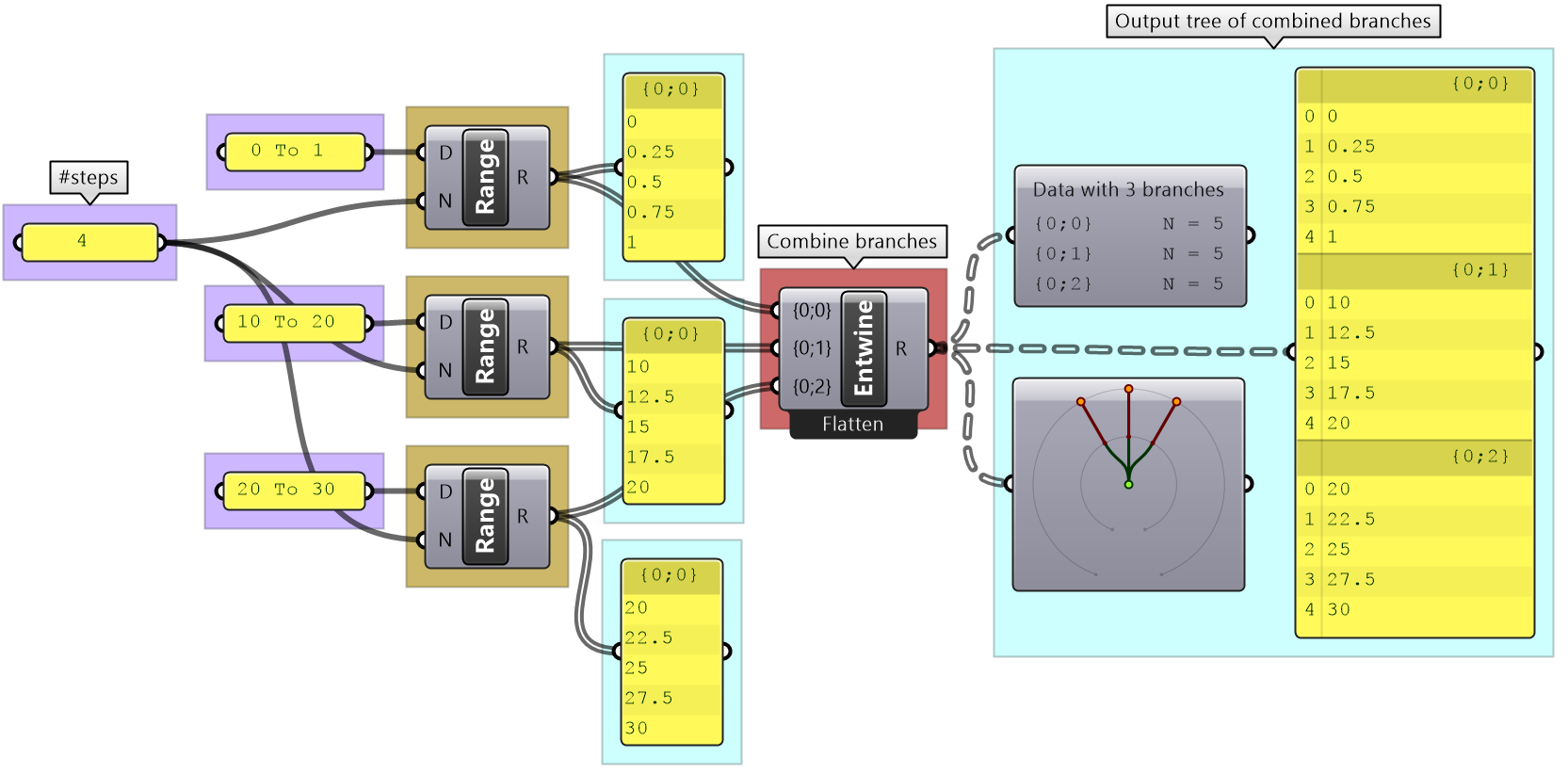
There are many components that generate data trees such as Grid and DivideSrf, and others that combine lists into a tree structure such as Entwine. Also all the components that produce lists can also create tree if the input is a list. For example, if input more than one curve into the DivideCrv component, we get a tree of points.
All components that generate lists of numbers (such as Range and Series) can also generate trees when given a list of input.
Perhaps one of the most common cases to generate a tree is when dividing a list of curves to generate a grid of points. So the input is one list and the output is a tree.
Generating trees tutorial
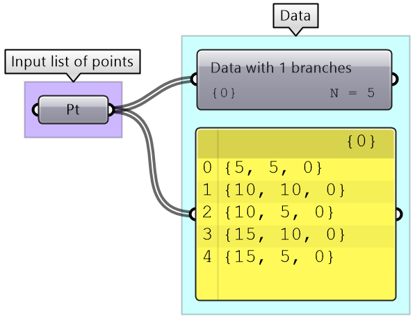
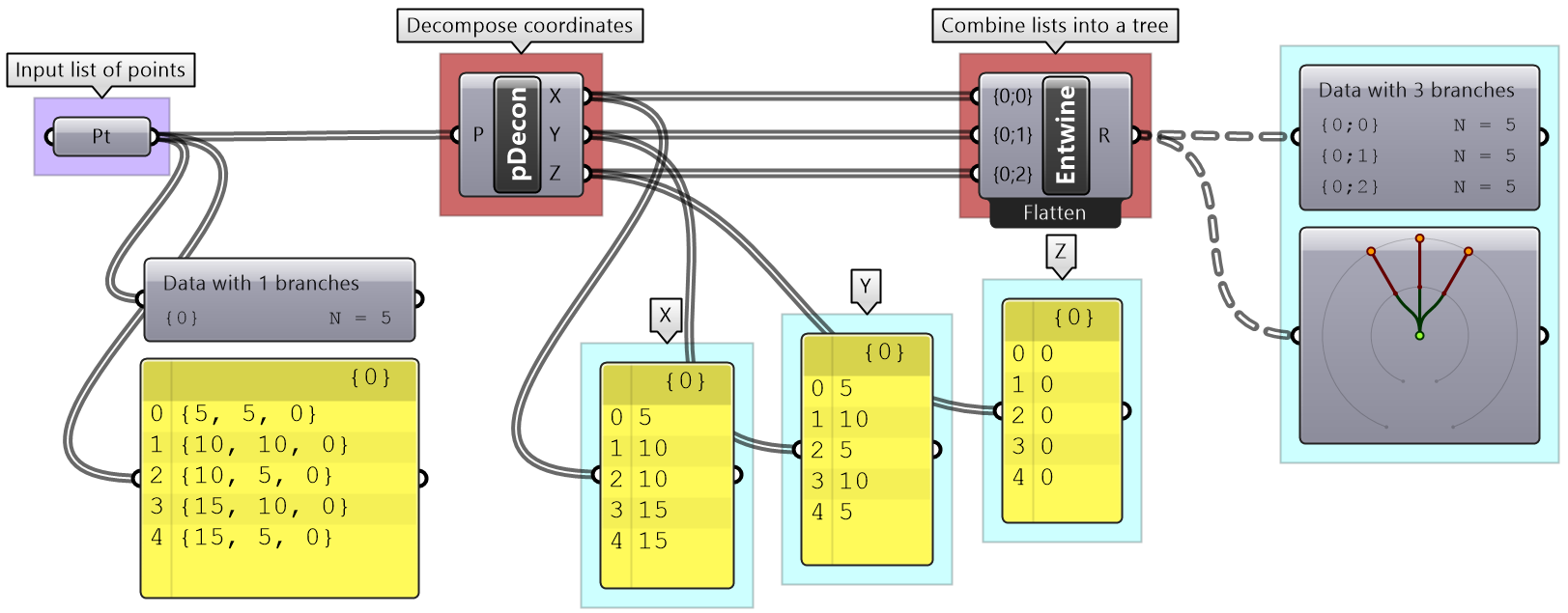
Given the following list of points, construct a number tree with 3 branches, one for each coordinate.
| Solution |
|---|
|
Discussion: Each input point is a single data item that contains 3 numbers (coordinates). We know we would like to isolate each coordinate into a separate list, then combine them into one data structure. Hence we need to first deconstruct input points (use Deconstruct of pDecon component), then combine the lists into one structure (use Entwine component). |
Tree matching
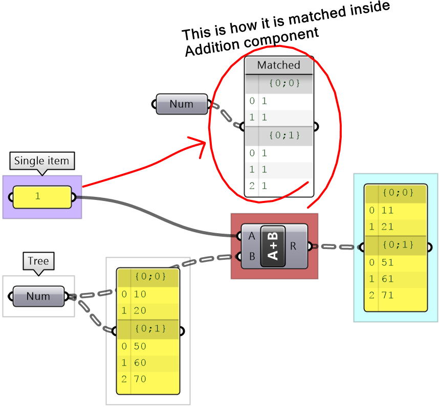
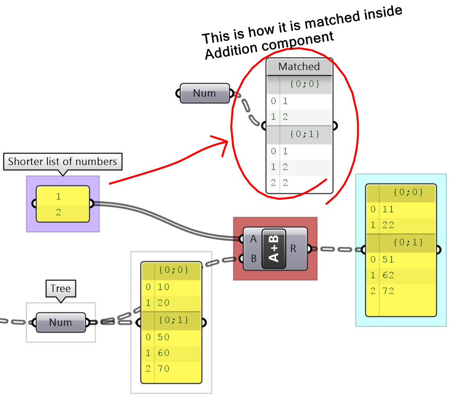
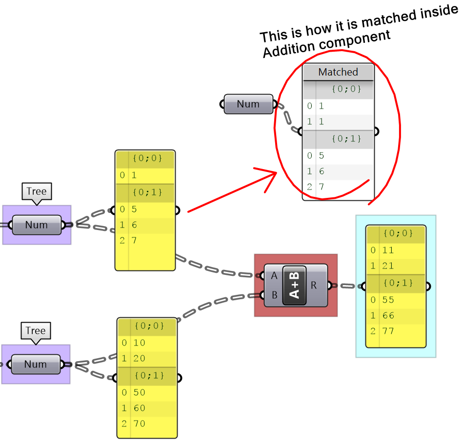
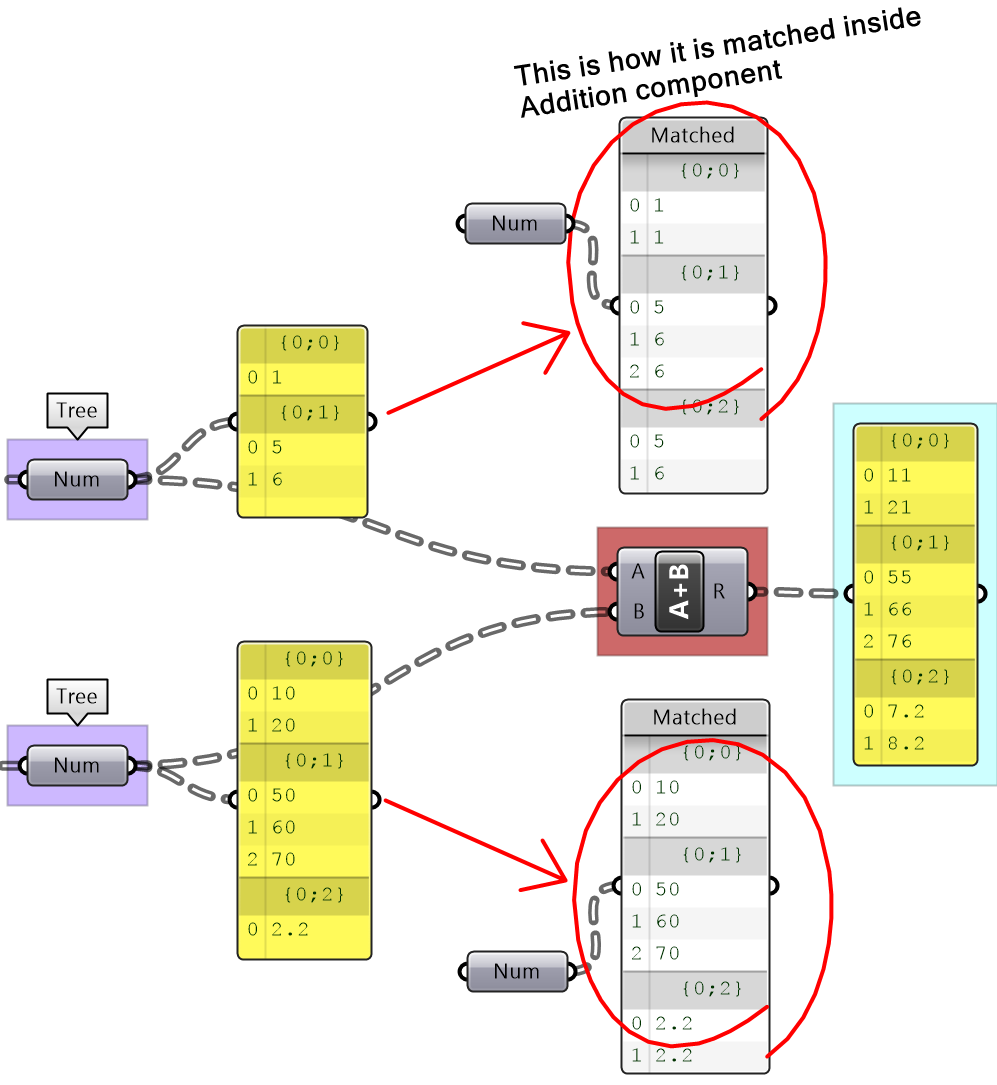
We explained the Long, Short and Cross matching with lists. Trees follow similar conventions to expand the shorter branches by repeating the last element to match. If one tree has less branches, the last branch is repeated. The following illustrates common tree matching cases.
| Demonstration | |
|---|---|
|
Matching an item with a tree. |
|
|
Matching a shorter list with a tree (tree branches longer than the list). |
|
|
Matching a longer list with a tree (tree branches shorter than the list). |
|
|
Match 2 trees with same number of branches. |
|
|
Match 2 trees with different number of branches. |
|
Tree matching tutorials
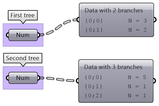
Inspect the following 2 number structures, then predict the structure and result of adding them (with default Grasshopper matching). Verify your answer using Addition components.
| Solution |
|---|
|
Key solution idea: The two input trees have different number of branches and different number of elements in each branch. The last branch of the shorter tree is repeated to match the number of branches, then corresponding branches are matched by repeating the last element of the shorter branch. |
Traversing trees
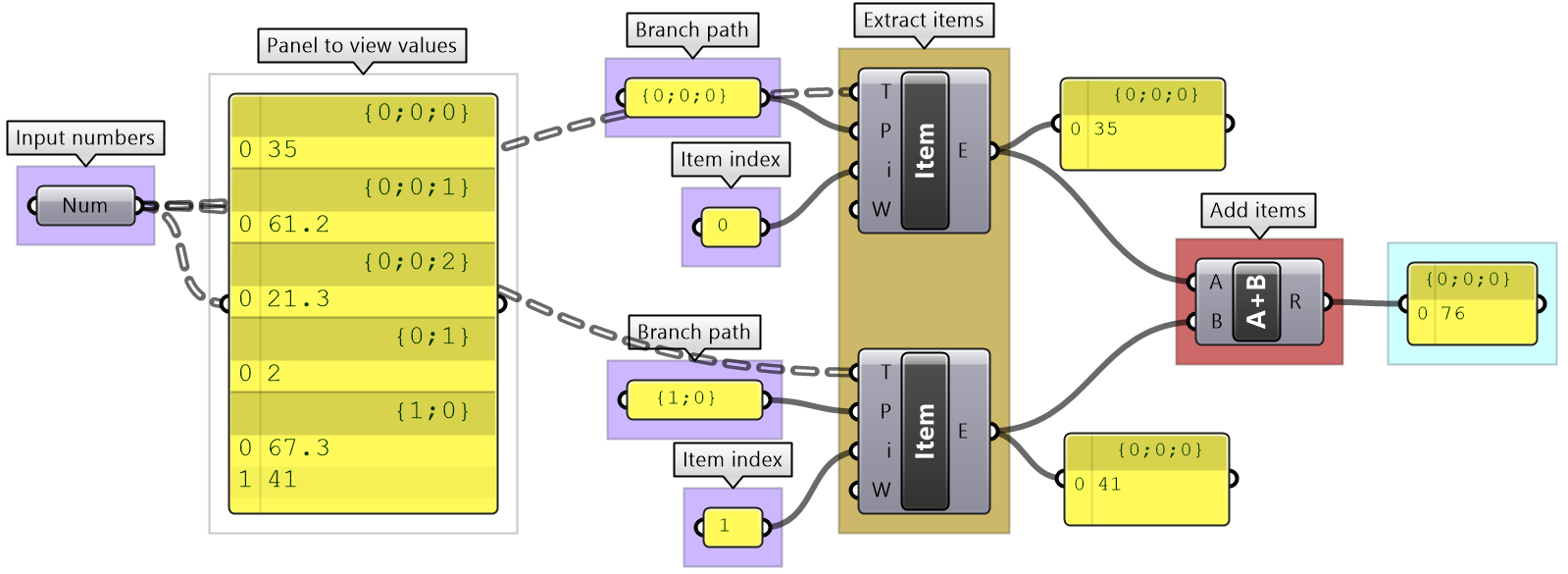
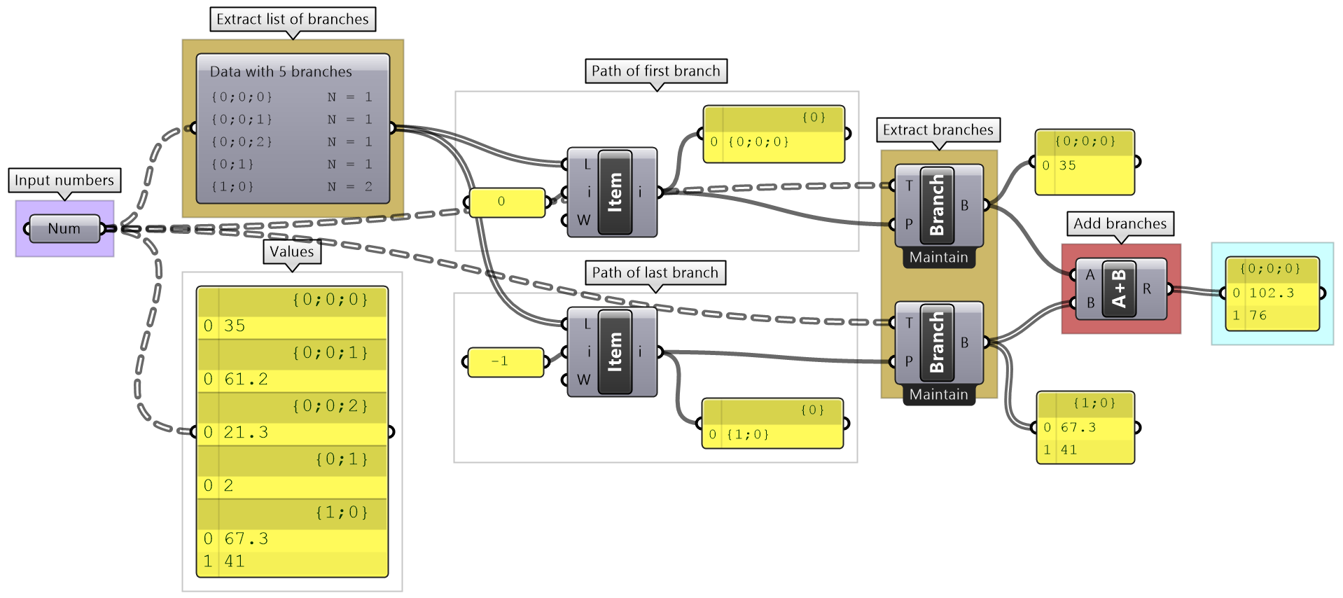
Grasshopper provides components to help extract branches and items from trees. If you have the path to a branch or to an item, then you can use Branch and Item components. You need to check the structure of your input so you can supply the correct path.
If you know that your structure might change, or you simply do not want to type the path, you can extract the path using the Param Viewer and List Item components.
Traversing trees tutorial
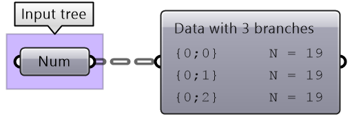
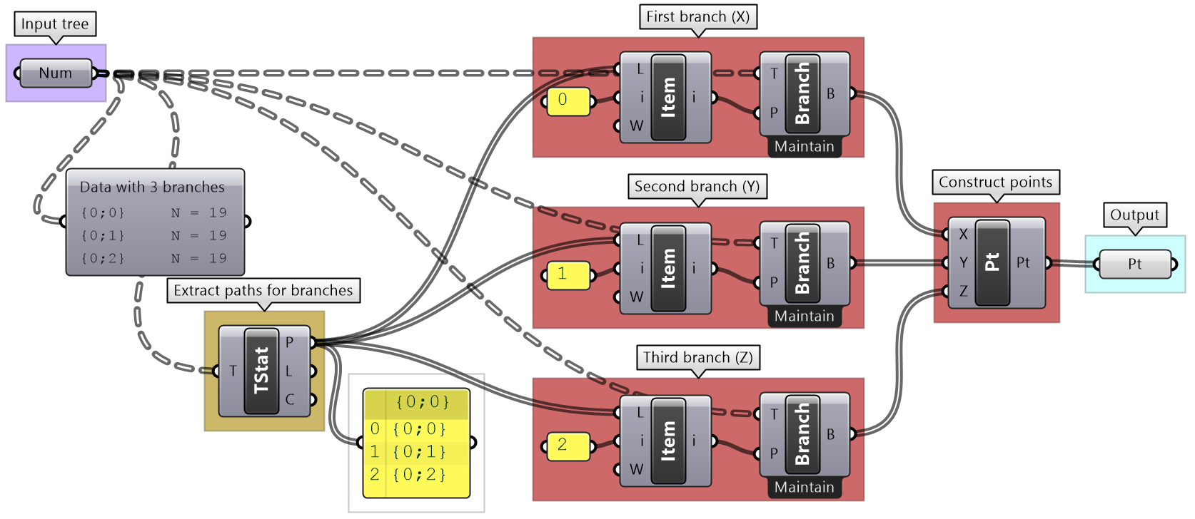
The following tree has 3 branches for each one of the coordinates (x, y, z) of some list of points. Use that tree to construct a list of these points.
| Solution |
|---|
|
Key solution idea: We can construct a point list using as input 3 lists representing X, Y and Z values. If we can isolate the 3 branches of the input tree, then we will be able to feed them to the point construction component. |
Basic tree operations
Basic tree operations are widely used and you will likely need them in most solutions. It is very important to understand what these operations do, and how they affect the output.
Viewing the tree structure
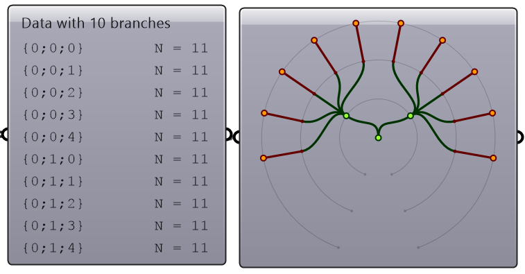
As we have seen in the data matching, different data structures of the same set of elements produce different results. Grasshopper offers three ways to view the data structure, the Parameter Viewer in text or diagram format, and the Panel.
Tree information can be extracted using the TStats component. You can extract the list of paths to all branches, number of elements in each branch and the number of branches.
List operations on trees
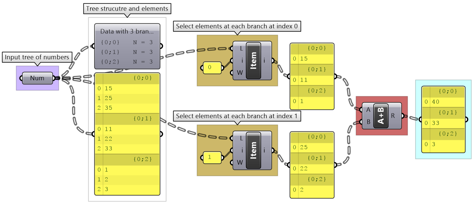
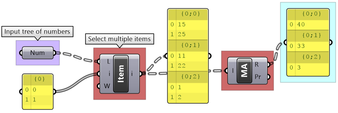
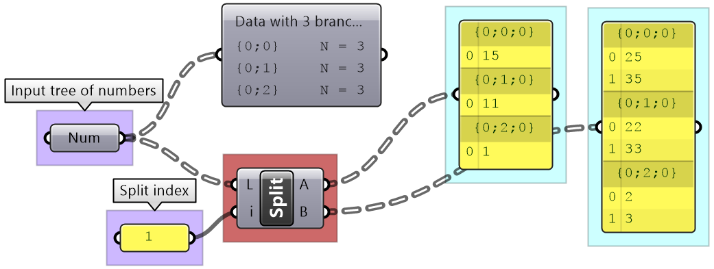
Trees can be thought of as a list of branches. When using list operations on trees, each branch is treated as a separate list and the operation is applied to each branch independently. It is tricky to predict the resulting data structure and therefore it is always important to check your input and output structures before and after applying any operation.
To illustrate how list operations work in trees, we will use a simple tree, a grid of points, and apply different list operations on it. We will then examine the output and its data structure.
| Operations | Example of how the list operation apply to trees. |
|---|---|
|
List Item: Select items at specific index in each branch. |
|
|
List Item: Select multiple indices to isolate part of the tree and perform one operation on such as Mass Addition. |
|
|
Split List: Split the elements of branches into 2 trees at the specified index. |
|
|
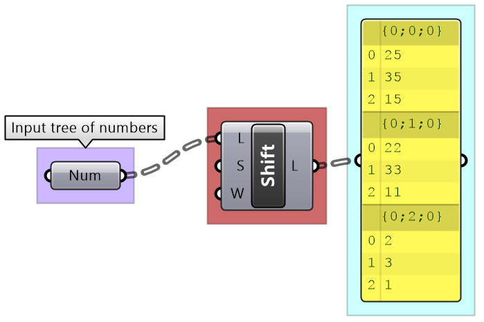
Shift List: Shifts the elements of each branch. |
|
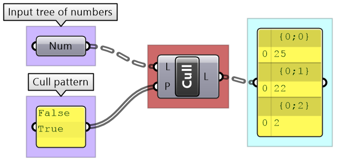
|
Cull Pattern: Culls each branch. |
Grafting from lists to a trees
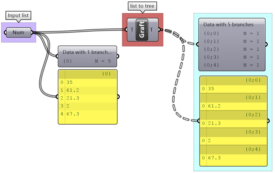
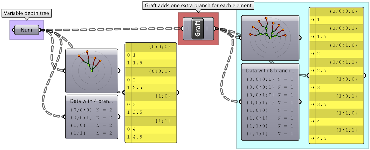
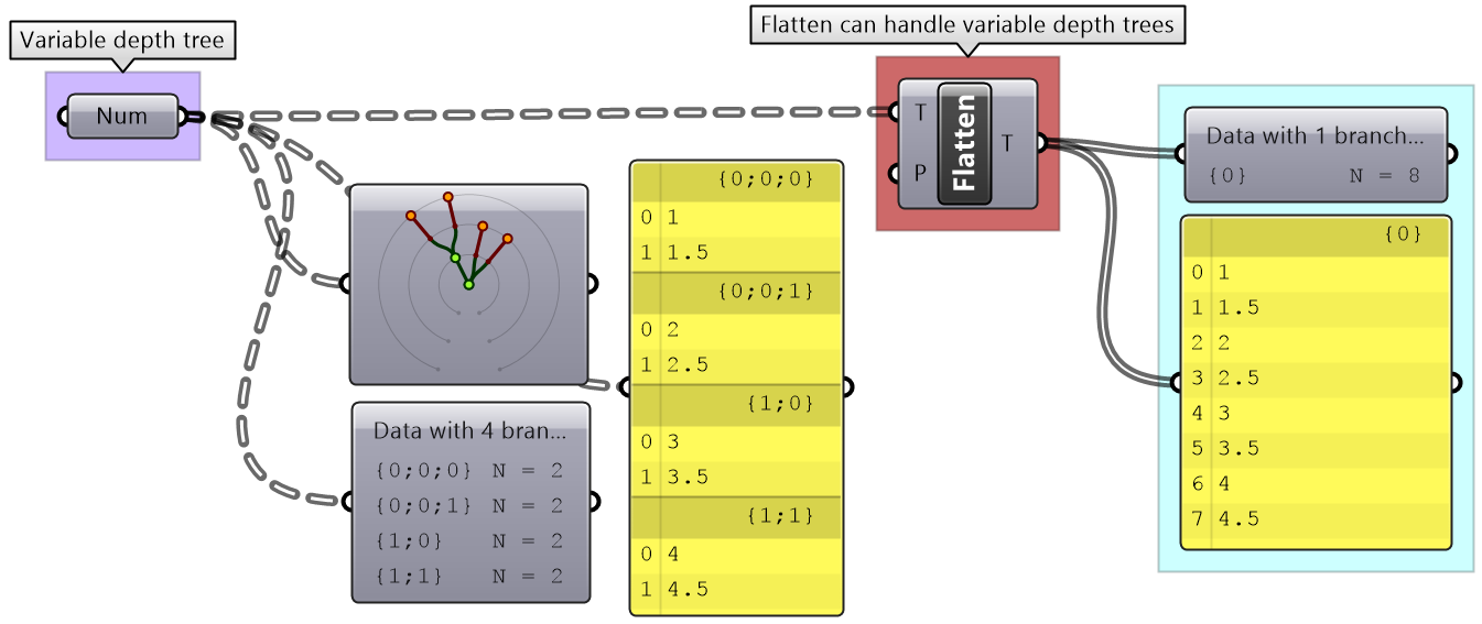
In some cases you need to turn a list into a tree where each element is placed in its own branch. Grafting can handle complex trees with branches of variable depths.
It might feel unintuitive to complicate the data structure (from a simple list to a tree), but grafting is very useful when trying to achieve certain matching. For example if you need to add each element of one list with all the elements in the second list, then you will need to graft the first list before inputting to the addition process.
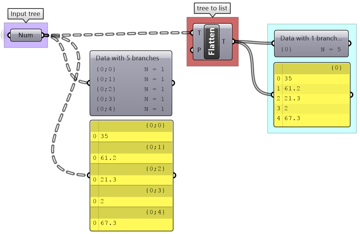
Flattening from trees to lists
Other times you might need to turn your tree structure into a simple list. This is achieved with the flattening process. Data from each branch is extracted and sequentially attached to one list.
Flatten also can handle any complex tree. It takes the branches in order starting with the lowest index trunk and put all elements in one list.
Combining data streams
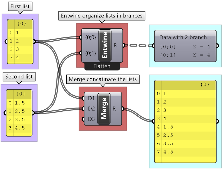
It is possible to compose a number of lists into a tree where each list becomes a branch in a new tree. It is different from the merging of lists where simply one bigger list is created.
Flipping the data structure
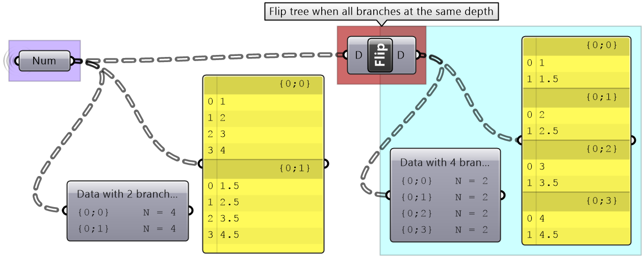
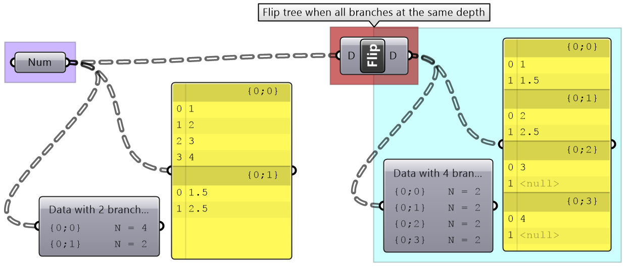
It is logical in some cases to flip the tree to change the direction of branches. This is especially useful in grids when points are organized in rows and columns (similar to a 2 dimensional array structure). Flipping causes corresponding elements across branches (have same index in their branch) to be grouped in one branch. For example, a data tree that has 2 branches and 4 items in each branch, can be flipped into a tree with 4 branches and 2 elements in each branch.
If the number of elements in the branches are variable in length, some of the branches in the flipped tree will have “null” values.
Flipping is one of the operations that cannot handle variable depth branches, simply because there is no logical solution to flip.
Simplifying the data structure
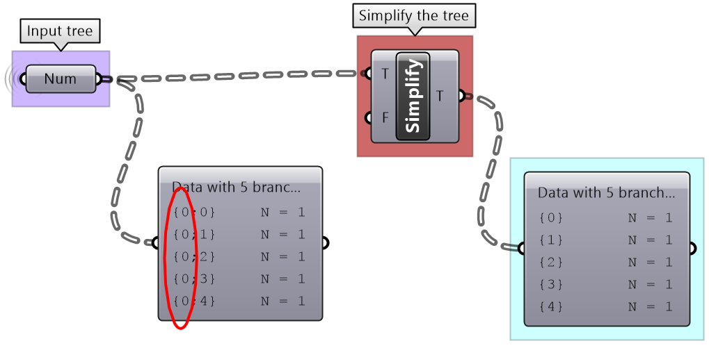
Processing data through multiple components can add unnecessary complexity to the data structure. The most common form is adding leading or trailing zeros to the paths addresses. Complex data structures are hard to match. Simplify Tree process helps remove empty branches. There are other operations such as Clean Tree and Trim Tree to help remove null elements, empty branches and reduce complexity. It is also possible to extract all branches as separate lists using Explode Tree operation.
Basic tree operations tutorial #1
| Solution | |
|---|---|
|
Input curve. Data structure: single item (one branch and one item in the branch) |
|
|
Divide curve to extract points. Data structure: list (one branch with 11 items). Note that the path has added leading “0”. This indicates the next layer of calculation. |
|
|
Create vertical lines at each point. Data structure: list (one branch with 11 items). Note that the path did not increase in complexity. |
|
|
Divide vertical lines to create a grid of points. Data structure: Tree (11 branches with 6 items). Note that the path has added leading “0”. |
|
|
Create horizontal lines at each point. Data structure: Tree (11 branches with 6 items). Note that the path did not increase in complexity. |
|
|
Create lofted surfaces through branches of lines. Data structure: Tree (11 branches with 1 item each). Note that the path did not increase in complexity. |
|
|
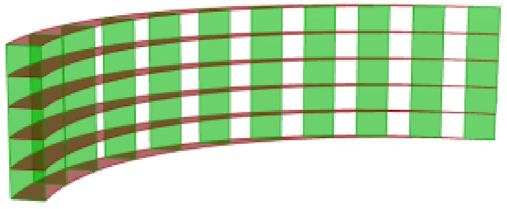
Flip the tree matrix and then create lofted surfaces through branches of lines. Data structure: Tree (11 branches with 1 item each). Note that the path did not increase in complexity. You can flatten the tree to create one list of horizontal louvers. |
|
Simple tree operations tutorial #2
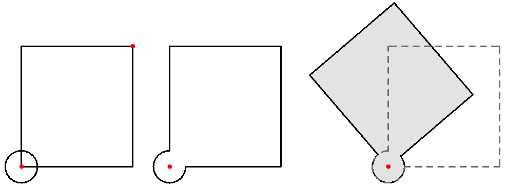
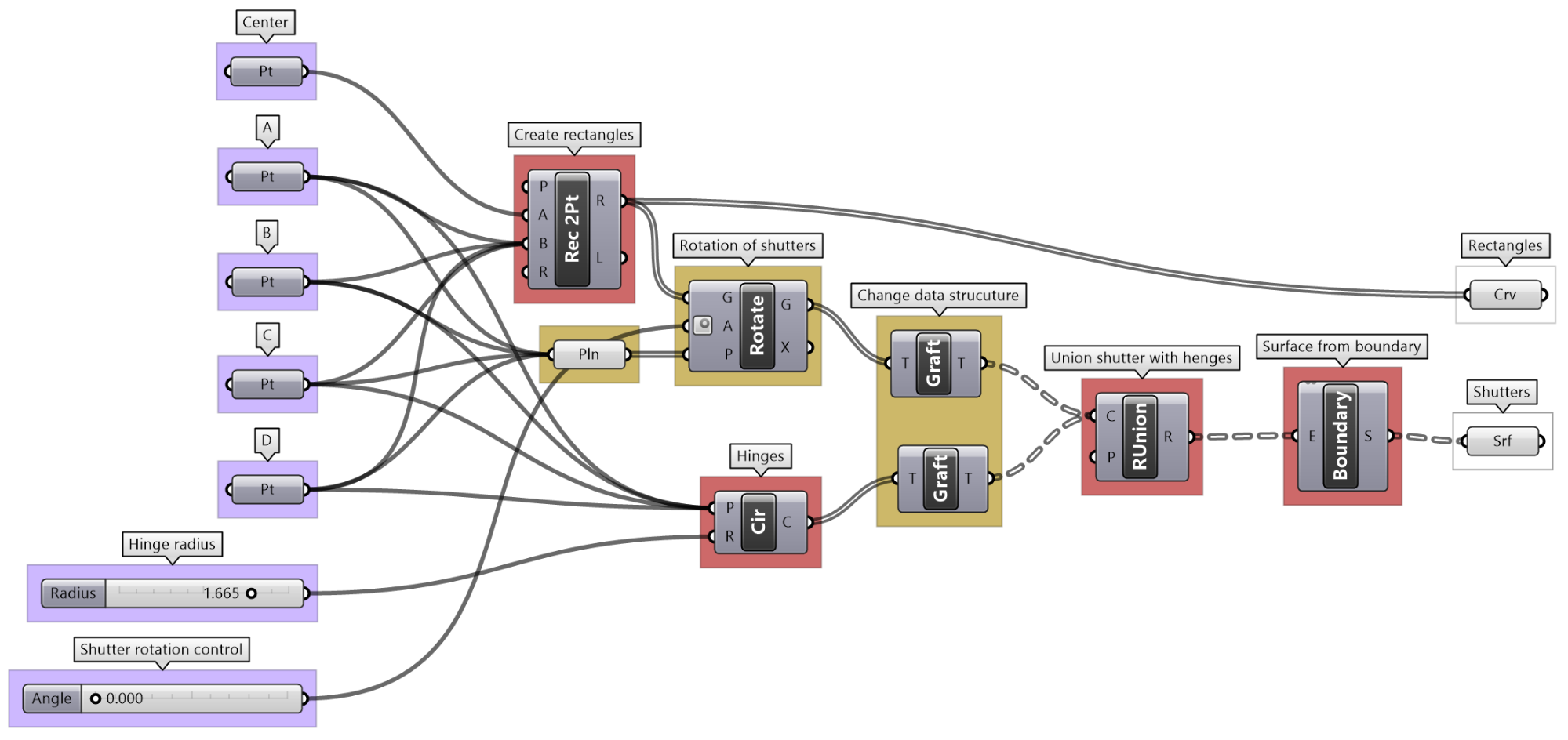
Given four corner points on a plane and a radius for the hinge, create a shutter that can open and shut as in the image using a rotation parameter.
| Algorithm Analysis | |
|---|---|
|
For each shutter there are two parts: the rectangle and the hinge. Union the rectangle and hinge, then allow rotating around the hinge. There is one rotation control to move all shutters together. |
|
| Grasshopper Implementation | |
|
Output Surface of the shutters. Curves for the frame. |
|
|
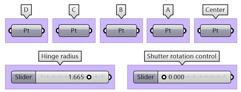
Input 4 corner points (and centre). Hinge radius. Rotation parameter. |
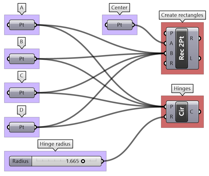
|
|
Key processes Create rectangle and hinges. Use Rectangle. |
|
|
Union the curves Use RUnion. Create a surface from the boundary. Use Boundary component. |
|
|
Intermediate process #1 Rotate the rectangles using the angle. Use Rotate component. |
|
|
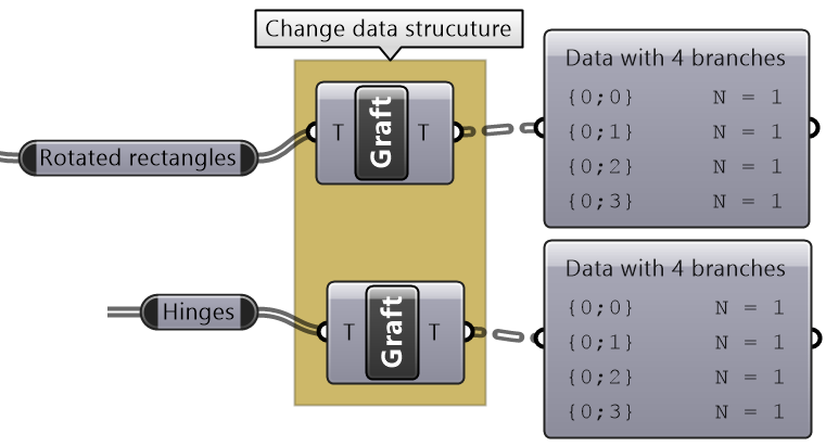
Intermediate process #2 Properly match the data structures of the rectangles and hinges before the region union. Use Graft so that rectangles and hinges pair correctly. |
|
| Put it all together. | |
Advanced tree operations
As your solutions increases in complexity, so will your data structures. We will discuss three advanced tree operations that are necessary to solve specific problems, or are used to simplify your solution by tabbing directly into the power of the data tree structure.
Relative items
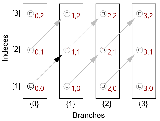
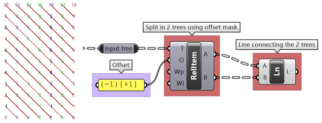
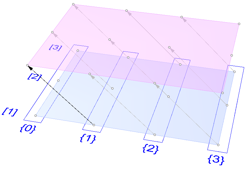
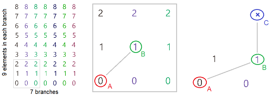
The first operation has to do with solving the general problem of connectivity between elements in one tree or across multiple trees. Suppose you have a grid of points and you need to connect the points diagonally. For each point, you connect to another in the +1 branch and +1 index. For example a point in branch {0}, index [0], connects to the point in branch {1}, index [1].
In Grasshopper, the way you communicate the offset is expressed with an offset string in the format “{branch offset}[index offset]”. In our example, the string to connect points diagonally is “{+1}[+1]”. Here is an example that uses relative tree component in Grasshopper. Notice that the relative item component creates two new trees that correlate in the manner specified in the offset string.
Here is an example implementation in Grasshopper where we define relative items in one tree, then connect the two resulting trees with lines using the Relative Item component.
Relative item tutorial #1
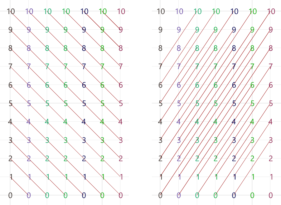
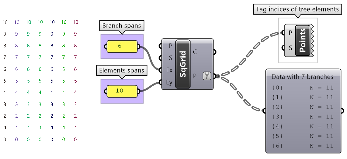
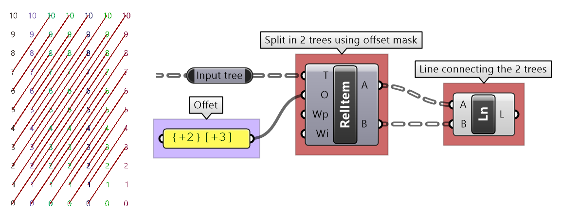
Create the pattern shown in the image using a square grid of 7 branches where each branch has 11 elements.
| Solution | |
|---|---|
|
Define the {branch_offset} [index_offset] | |
|
Create the grid |
|
|
Create relative trees that connect each element with -1 branch and +1 index: {-1}[+1] Create lines to connect the 2 relative trees. |
|
|
Change the offset to {+2}[+3] to create the second connections. |
|
We showed how to define relative items in one tree, but you can also specify relative items between 2 trees. You’ll need to pay attention to the data structure of the two input trees and make sure they are compatible. For example, if you connect each point from the first tree with another point from a different tree with the same index, but +1 branch, then you can set the offset string to be {+1}[0].
The input to the Relative Items component is two trees and the output is two trees with corresponding items according to the offset string.
The following GH definition achieves the following:
Relative item tutorial #2
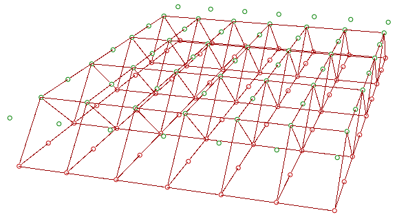
Use relative items between 2 bounding grids to generate the structure shown in the image.
| Solution | |
|---|---|
|
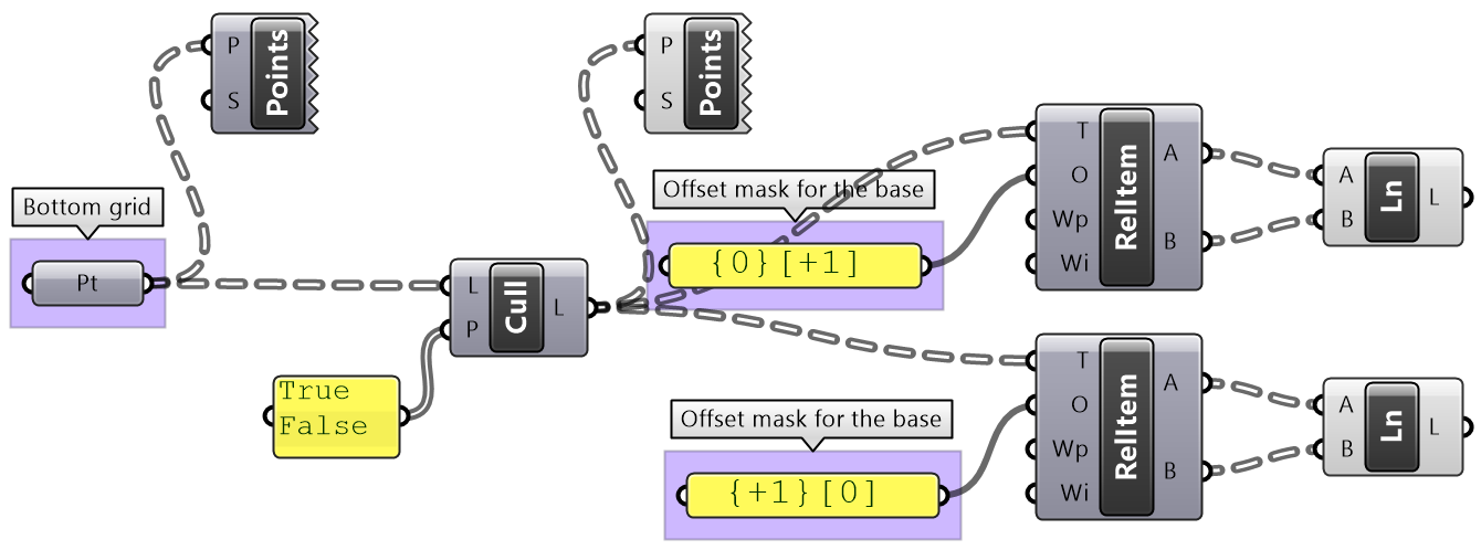
Bottom tree connections | |
|
Cull every other index and keep the same number of branches (cull inices 1, 3,...). Define the offset strings for RelativeItem components to create the vertical and horizontal connections. |
|
|
Grasshopper definition |
|
|
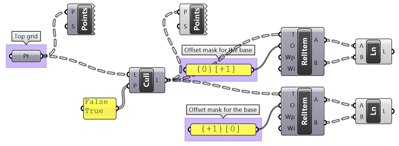
Top tree connections | |
|
Cull every other index and keep the same number of branches (cull inices 0, 2,...) Define the offset strings for RelativeItem components to create the vertical and horizontal connections |
|
|
Grasshopper definition |
|
|
Connections between the 2 trees | |
|
Use culled grids, then define first offset string for RelativeItems component to create the first set of cross lines: {0}[0]. |
|
|
Define second offset string for RelativeItems component to define the second set of cross lines: {0}[-1]. |
|
Split trees
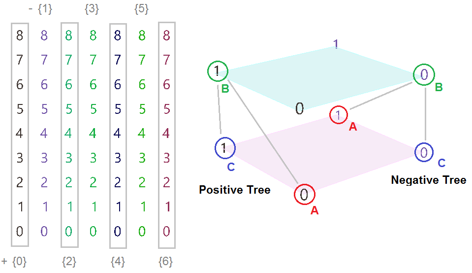
The ability to select a portion of a tree, or split into two parts is a very powerful tree operation in Grasshopper. You can split the tree using a string mask that specifies the positive output of your tree, and what’s left is called the negative tree and is given as an output. Since all trees are made out of branches and indices, the split mask should include information about which branches and indices within these branches to split. Here are the rules of the split mask.
| Split tree mask: syntax and general rules | |
|---|---|
| { ; ; } | Use curly brackets to enclose the mask for the tree branches. |
| [ ] | Use square brackets to enclose the mask for the elements (leaves), inside square brackets. Can omit if select all items or use [*]. |
| ( ) | Round brackets are used for organizing and grouping. |
| * | Any number of integers in a path. The asterisk also allows you to include all branches, no matter what their paths look like. |
| ? | Any single integer. |
| 6 | Any specific integer. |
| !6 | Anything except a specific integer. |
| (2,6,7) | Any one of the specific integers in this group. |
| !(2,6,7) | Anything except one of the integers in this group. |
| (2 to 20) | Any integer in this range (including both 2 and 20). |
| !(2 to 20) | Any integer outside of this range. |
| (0,2,...) | Any integer part of this infinite sequence. Sequences have to be at least two integers long, and every subsequent integer has to be bigger than the previous one (sorry, that may be a temporary limitation, don't know yet). |
| (0,2,...,48) | Any integer part of this finite sequence. You can optionally provide a single sequence limit after the three dots. |
| !(3,5,...) | Any integer not part of this infinite sequence. The sequence doesn't extend to the left, only towards the right. So this rule would select the numbers 0, 1, 2, 4, 6, 8, 10, 12 and all remaining even numbers. |
| !(7,10,21,...,425) | Any integer not part of this finite sequence. |
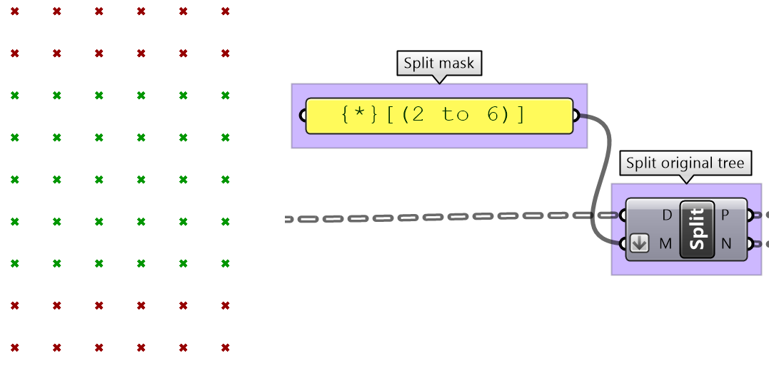
| { * }[ (0 to 4) or (6,11,41) ] | It is possible to combine two or more rules using the boolean and/or operators. The example selects the first five items in every list of a tree and also the items 7, 12 and 42, then the selection rule. |
Here are some examples of valid split masks.
|
Split by branches | |
| { * } | Select all (the whole tree output as positive, and negative tree will be empty). |
| { *; 2 } | Select the third branch. |
| { *; (0,1) } | Select the first two end branches. |
| { *; (0, 2, …) } | Select all even branches. |
|
Split by branches and leaves | |
| { * }[(1,3,...)] | Select elements located at odd indices in all branches. |
| { *; 0 }[(1,3,...)] | Select elements located at odd indices in the first branch. |
| { *; (0, 2) }[(1,3,...)] | Select elements located at odd indices in the first and third branches. |
| {*; (0,2,...) } [ (1,3,...) ] | Select elements located at odd indices in branches located at even indices. |
| {*; (0,2,...) } [(0) or (1,3,...)] | Select elements located at odd indices, and index “0”, in branches located at even indices. |
One of the common applications that uses split tree functionality is when you have a grid of points that you like to transform a subset of it. When splitting, the structure of the original tree is preserved, and the elements that are split out are replaced with null. Therefore, when applying transformation to the split tree, it is easy to recombine back.
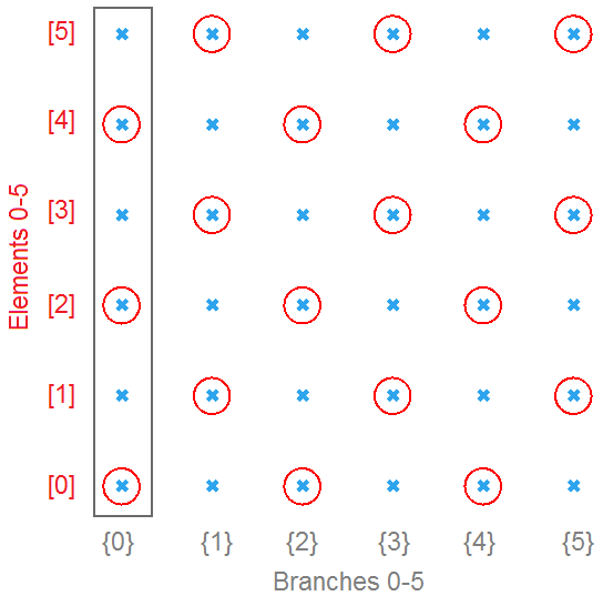
Suppose you have a grid with 7 branches and 11 elements in each branch, and you’d like to shift elements between indices 1-3 and 7-9. You can use the split tree to help isolate the points you need to move using the mask: {*}[ (1,2,3) or (7,8,9) ], move the positive tree, then recombine back with the negative tree.
This is the GH definition that does the above using the Split Tree component.
One of the advantages of using Split Tree over relative trees is that the split mask is very versatile and it is easier to isolate the desired portion of the tree. Also the data structure is preserved across the negative and positive trees which makes it easy to recombine the elements of the tree after processing the parts.
Split tree tutorial #1
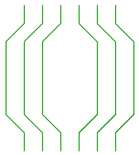
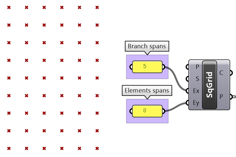
Given a 6x9 grid, use the split tree to generate the following form.
| Solution steps | |
|---|---|
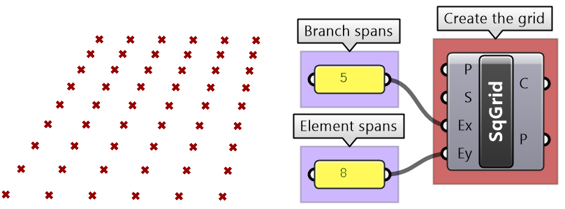
| Create the grid. | |
| Split the tree to isolate the middle part. | |
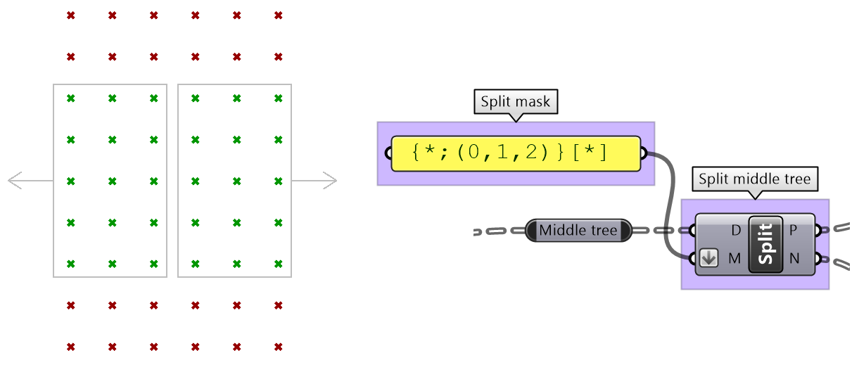
| Split the middle part into two new parts. | |
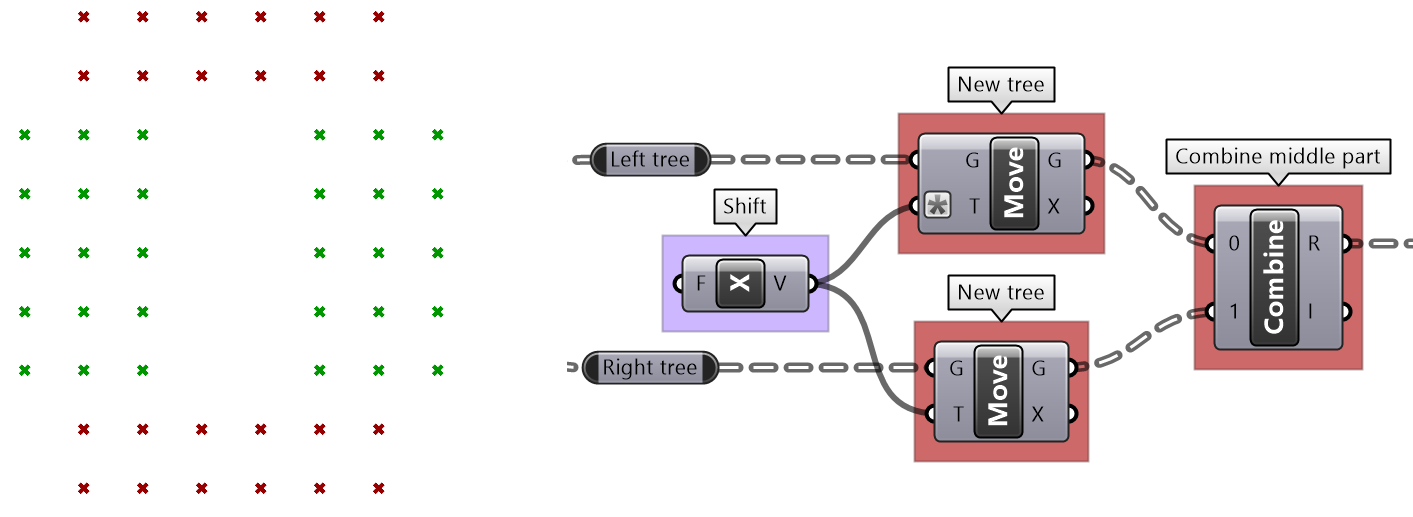
| Move the two middle parts in opposite directions then recombine them. | |
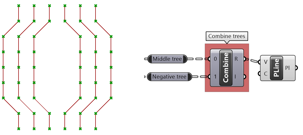
| Recombine the middle part with the rest of the tree and create polylines through each branch elements. | |
Split tree tutorial #2
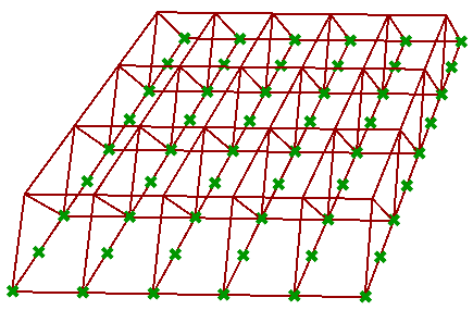
Given a grid, create the following truss system using split tree functionality.
| Solution | |
|---|---|
| Create the 6x9 grid. | |
| Split at every other element. | |
| Move positive tree vertically. | |
| Combine positive and negative trees and create a polyline through each branch elements | |
| Create bottom curves using negative tree. | |
| Create top curves using positive tree. | |
Path mapper
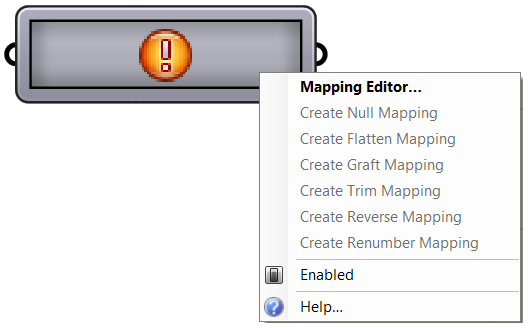
When dealing with complex data structures such as the Grasshopper data trees, you’ll find that you need to simplify or rearrange your elements within the tree. There are a few components offered in Grasshopper for that purpose such as Flatten, Graft or Flip. While very useful, these might not suffice when operating on multiple trees or needing custom rearrangement. There is one very powerful component in Grasshopper that helps with reorganizing elements in trees or change the tree structure called the Path Mapper. It is perhaps the least intuitive to use and can cause a loss of data, but it is also the only way to find a solution in some cases, and hence it pays to address here.
The Path Mapper maps data between source and target paths. The source path is fixed, and is given by the input tree. You can only set the target path. There is a set of constants that help with the mapping. Here is a list of those.
| item_count | Number of items in the current branch |
| path_count | Number of paths (branches) in the tree |
| path_index | Index of the current path |
Let’s start by familiarizing ourselves with the syntax using built-in mappings inside the Path Mappers.
In the following example, the input tree has two grids of points (2 trees). The data structure becomes clear when using a Polyline which creates one polyline through each branch. We will examine the effect of applying the built-in mapp on the structure and connection of points.
| Built-in mappings inside the Path Mapper | |
|---|---|
|
Null Mapping |
Does not change anything. |
| Flatten Mapping | |
| Graft Mapping | |
| Reverse Mapping | |
| Renumbering Mapping | |
Path mapper tutorial #1
Given the tree structures of points, create the following connections.
| Solution | |
|---|---|
|
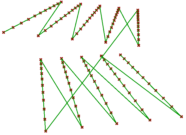
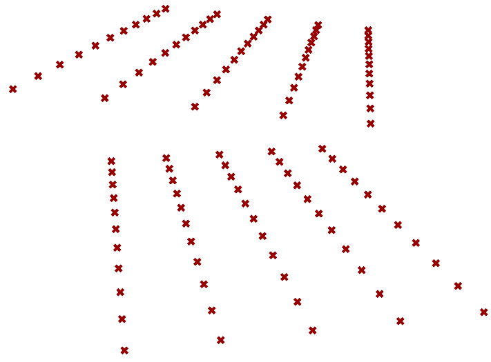
The input has two trees, and each has 5 branches with 11 elements in each branch, a total of 10 branches. |
|
|
A Polyline can be used to connect the elements in each branch. |
|
|
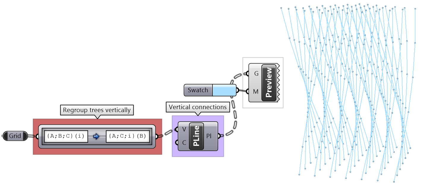
To create the vertical connections, you need to create a branch for each 2 corresponding elements across the 2 trees, then use Polyline to connect them. 1. Analyze the paths of the trees 2. Come up with a mapping that generates the desired grouping | |
|
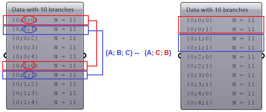
First, group corresponding branches across the 2 trees. That can be achieved by switching the last two integers in the paths: |
|
|
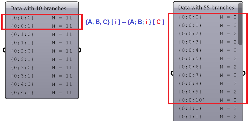
Second, Flip each of the 5 trees. Since the branches has 11 elements each, flipping each tree will create 11 branches with 2 elements in each branch. Total of 55 branches. You flip by switching the last integer of the path with the element index: |
|
|
Finally, a Polyline makes the vertical connections. Note: You can combine the 2 mappings in one step as in the following: Combining is not always possible, but it can save processing time and size. |
|
Path mapper tutorial #2
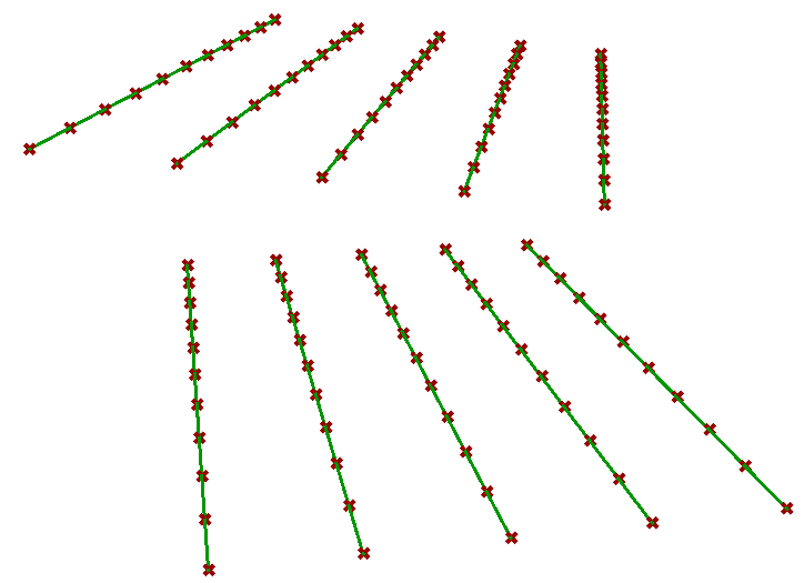
Given the input tree of points, create the following structure.
| Solution | |
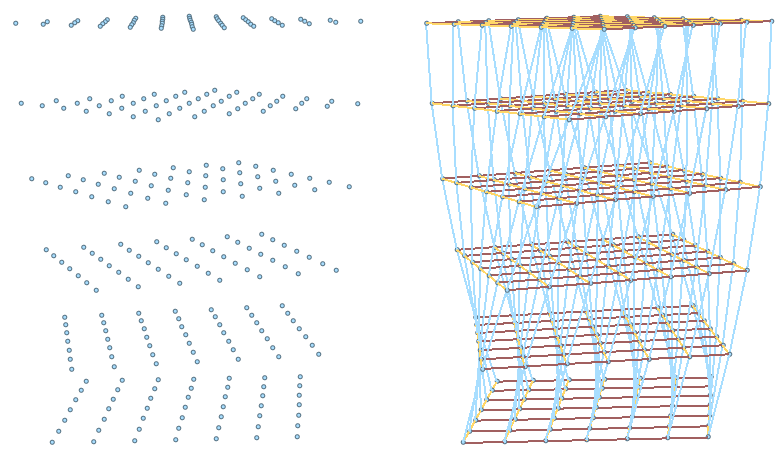
|---|---|
|
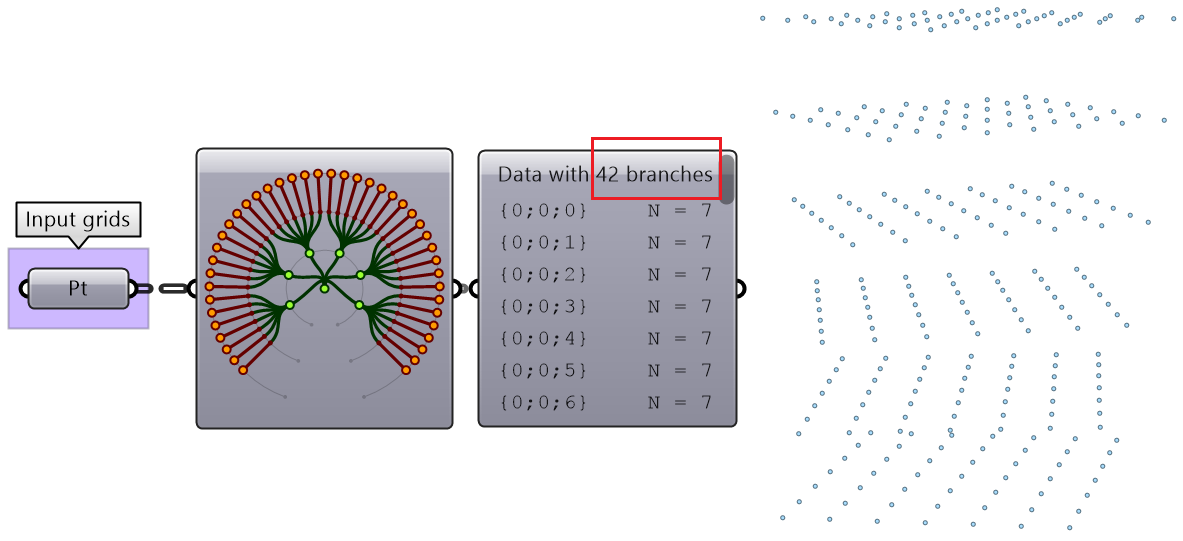
The initial tree has 42 branches, 7 branches in each of the 6 trees. |
|
|
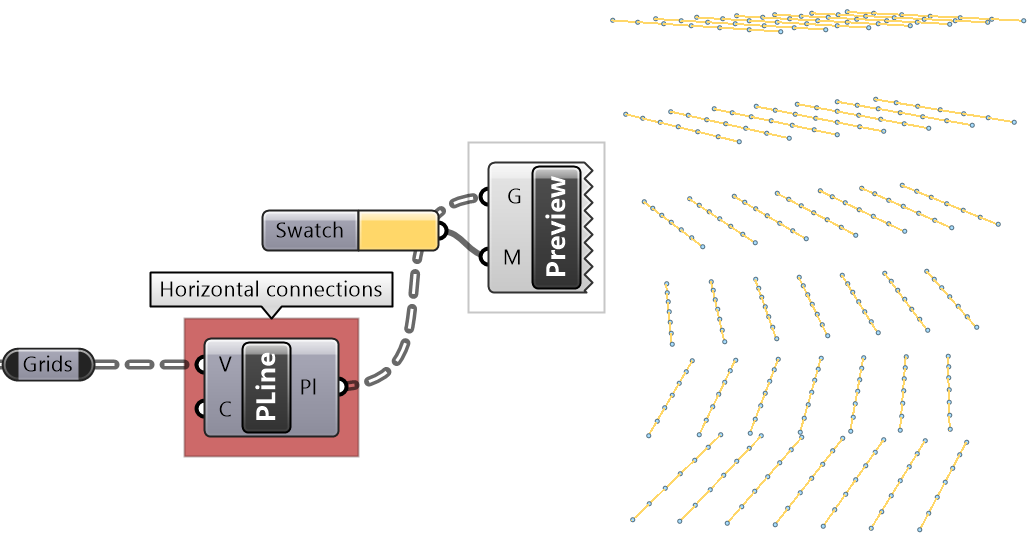
The Polyline component connects the elements in each branch. |
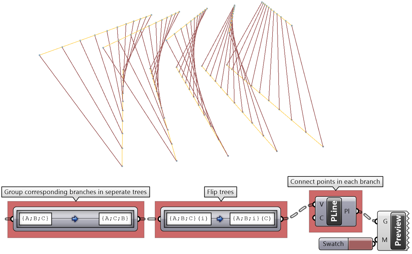
|
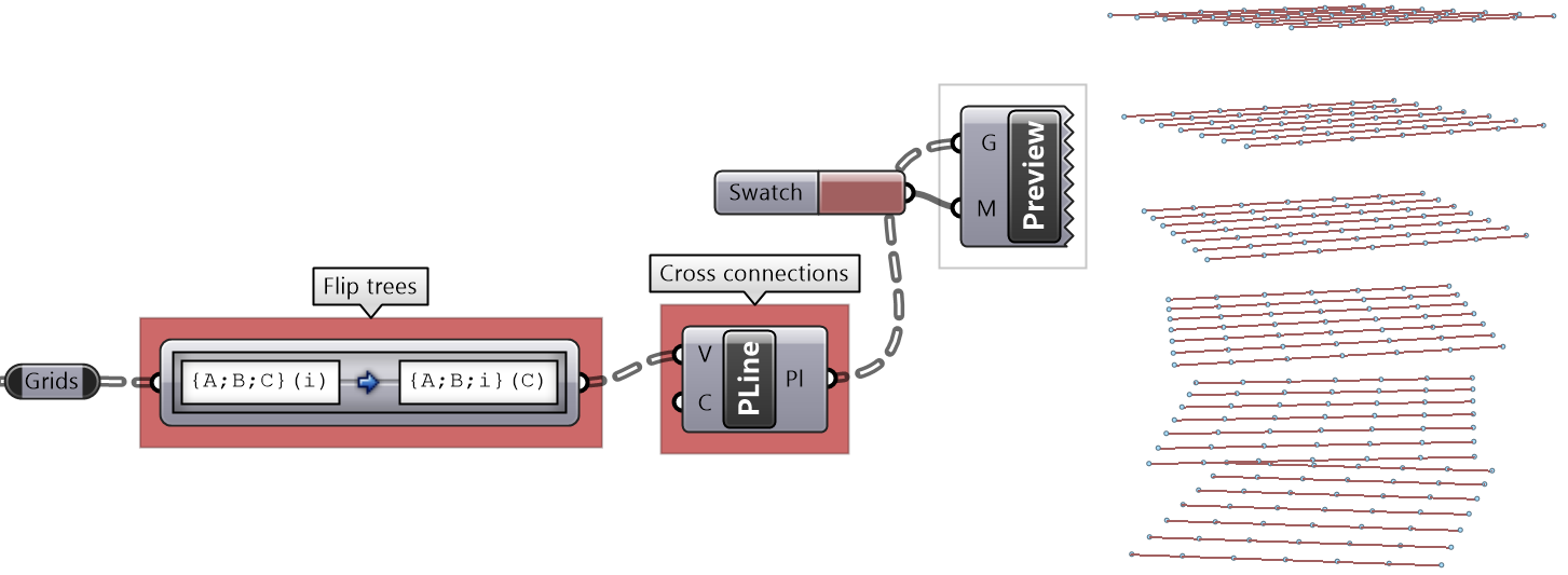
|
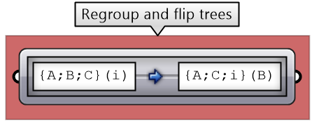
Flip the trees using Path Mapper by switching branch and element indices. |
|
|
Regroup the elements of corresponding branches in all trees using the Path Mapper. |
|
|
Final result Create all connections. |
|
Advanced data structures tutorials
Sloped roof tutorial
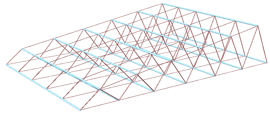
Create a parametric truss system that changes gradually in height as shown in the image.
| Solution | |
|---|---|
| Algorithm analysis | |
|
First, solve for one simple truss. | |
|
Identify desired output for a single truss. |
|
|
Define initial input 1. Base line on XY-Plane 2. Number of runs 3. Height |
|
|
Identify algorithms steps. | |
|
Create input (L=line, H=height and R= #runs). |
|
|
Divide curve by 2*R. |
|
|
Move every other point in the Z direction by height. |
|
|
Create 3 sets of ordered points for the bottom beams, top beams and middle beams, then connect each of the 3 sets with a polyline. |
|
| Implement the algorithm in Grasshopper. | |
|
Resolve for multiple trusses with variable height. | |
|
Create a series of base lines using the initial line and copy in Y-Axis direction. |
|
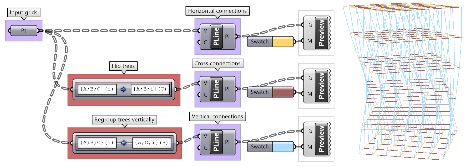
|
Use the list of lines as input instead of a single line. Notice that instead of a list of points for each of the 3 sets (bottom, top and middle), we now have a tree or grid of points with a number of branches equal to the number of trusses. |
|
|
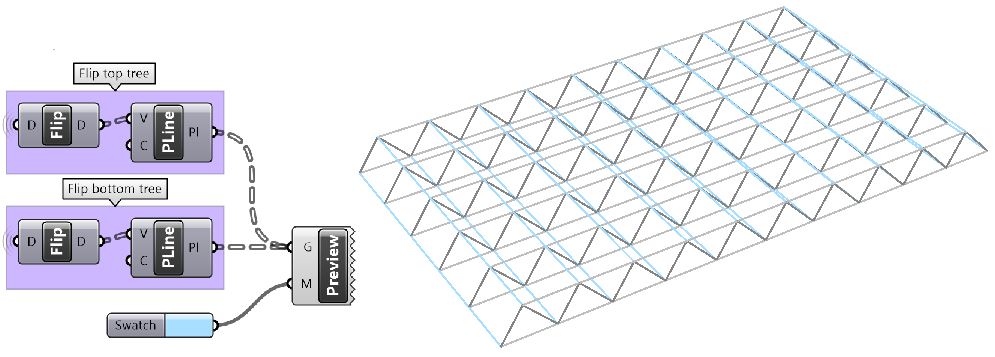
Create cross connections using Flip tree operation for the bottom and top trees. |
|
|
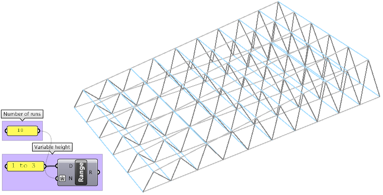
Create variable height. |
|
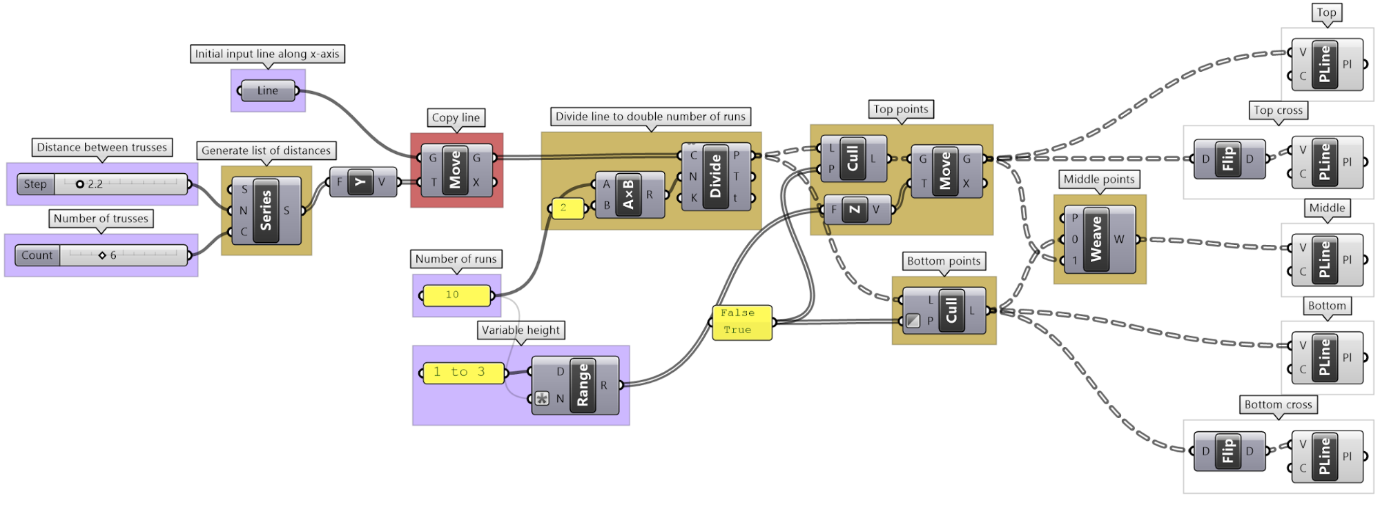
| The complete solution implementation in Grasshopper. | |
Diagonal triangles tutorial
Given the input grid, use the RelativeItem component to create diagonal triangles.
| Solution | |
|---|---|
| Algorithm analysis | |
|
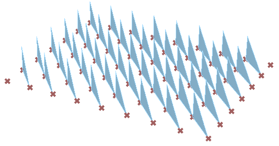
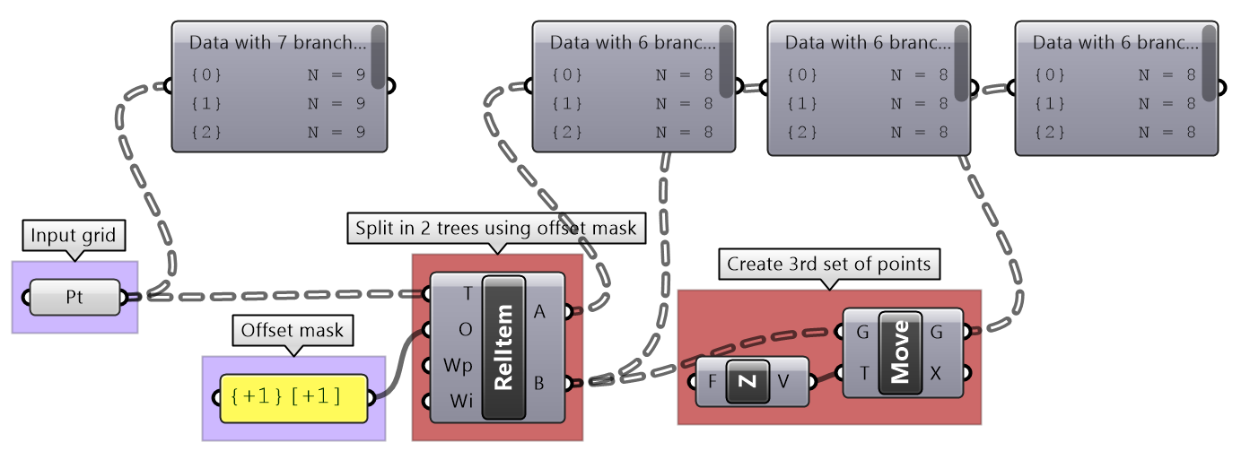
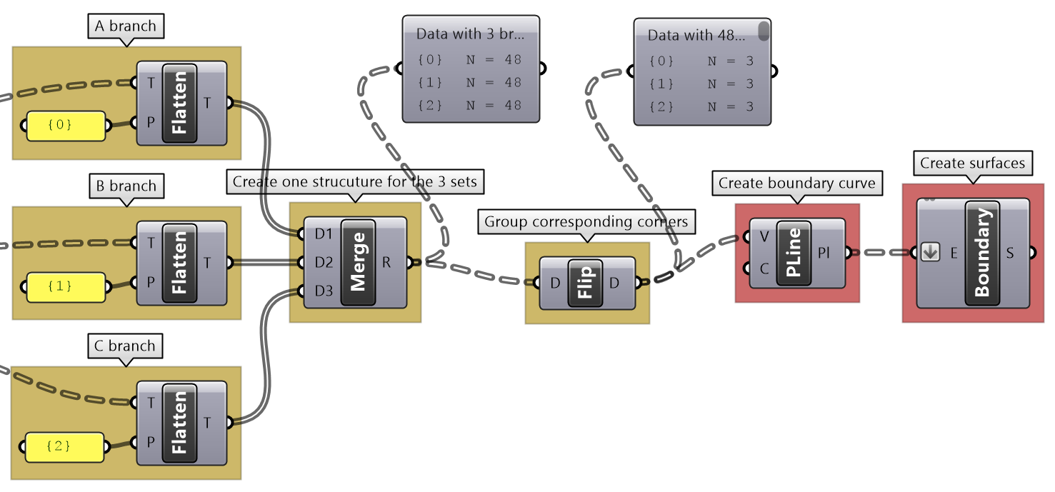
To generate the triangles, we need 3 sets of corner points. Two of the point sets (A, B) are within the grid. B is diagonal from A (relative index is +1 branch and +1 element). The third point set (C) is a copy of set (B) moved vertically. Group corners to connect into boundaries then generate surfaces. |
|
| Grasshopper implementation | |
|
Use RelativeItem to create set A and set B (use “{+1}[+1] mask). Move set B vertically. |
|
|
Use RelativeItem to create set A and set B (use “{+1}[+1] mask). Move set B vertically. |
|
Zigzag tutorial
Create the structure shown in the image using a base grid as input.
| Solution | |
|---|---|
| Algorithm analysis | |
|
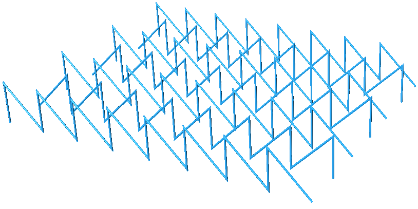
Since the zigzags alternate directions, it is best to split the grid into 2 parts, positive and negative. Find 3 sets of points in the positive tree and order. Reverse the elements in the branches of the negative tree, then find the 3 sets of points and order. Merge back the 2 trees to create geometry through points. |
|
| Grasshopper implementation | |
|
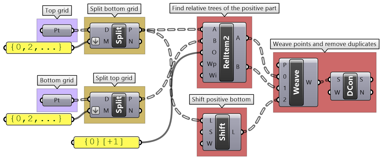
Use the Split Tree component to generate positive and negative trees for both bottom and top grids. Use {0,2,...} split mask. Use RelativeItems2 to create A and B trees, use {0}[+1] relative mask. Use Shift to create the C tree. Weave data together and remove duplicates. |
|
|
Merge ordered positive and negative trees to generate geometry using Polyline and Pipe components. |
|
Weaving tutorial
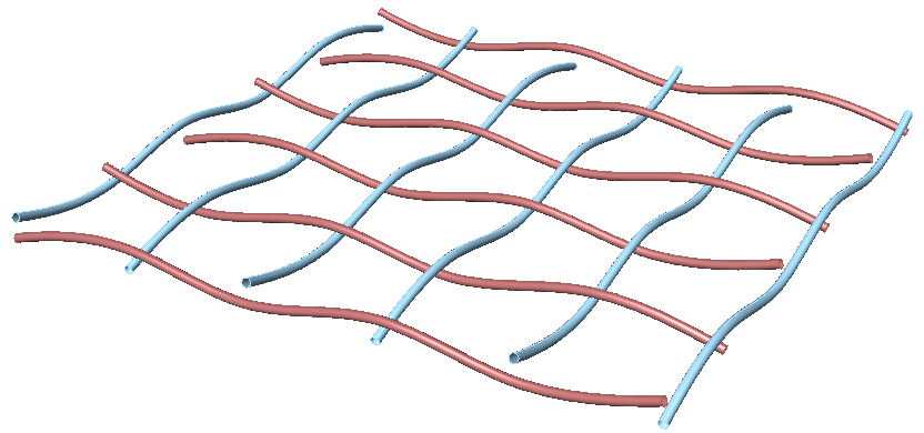
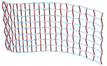
Create flat weaved threads using a rectangular grid as an initial input. Set your desired density and size. Bonus: Make the weaving go along any surface.
| Solution | |
|---|---|
| Algorithm analysis | |
|
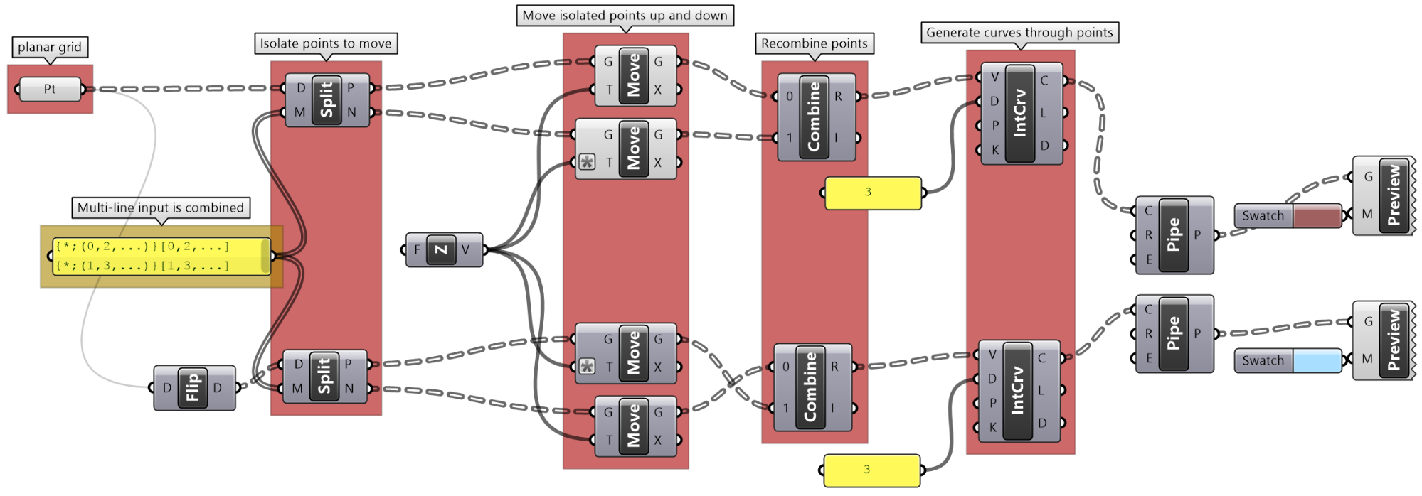
The input is a planar square grid with vertical branches. For vertical threads: Split the grid into two parts alternating elements in each branch. Move the first part up, and the second down, then recombine the parts into one set. Draw a curve through the points in each branch. Flip the grid, then repeat to create horizontal curves. |
|
| Grasshopper implementation | |
|
Use Split tree to separate alternating points and move up and down. Combine points and use IntCrv to interpolate through points of each branch. Flip the tree, and repeat Split, Combine and IntCrv to create curves in the other direction. |
|
| The full Grasshopper solution | |
| Bonus solution | |
|---|---|
|
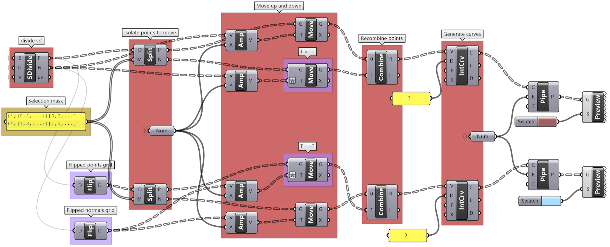
Instead of using the Z-Axis to move points up and down, use the surface normal direction at each point. Note: Make sure the data structure of normals and points match. | |
